The Generic Mapping Tools

Version 4.5.18
Technical Reference and Cookbook
by
Pål (Paul) Wessel
School of Ocean and Earth Science and Technology
University of Hawai’i at Mānoa
and
Walter H. F. Smith
Laboratory for Satellite Altimetry
NOAA/NESDIS/STAR
July 2018

Contents
Front page
List of Tables
List of Figures
Acknowledgments
The GMT Documentation Project
A Reminder
Copyright and Caveat Emptor!
Typographic conventions
1 Preface
1.1 What is new in GMT 4.x?
1.1.1 Overview of GMT 4.5.18 [Jul-1, 2018]
1.1.2 Overview of GMT 4.5.17 [Jan-1, 2018]
1.1.3 Overview of GMT 4.5.16 [June-25, 2017]
1.1.4 Overview of GMT 4.5.15 [October-1, 2016]
1.1.5 Overview of GMT 4.5.14 [Nov-1, 2015]
1.1.6 Overview of GMT 4.5.13 [Jan-1, 2015]
1.1.7 Overview of GMT 4.5.12 [Mar-1, 2014]
1.1.8 Overview of GMT 4.5.11 [Nov-5, 2013]
1.1.9 Overview of GMT 4.5.9 [Jan-1, 2013]
1.1.10 Overview of GMT 4.5.8 [Apr-1, 2012]
1.1.11 Overview of GMT 4.5.7 [Jul-15, 2011]
1.1.12 Overview of GMT 4.5.6 [Mar-1, 2011]
1.1.13 Overview of GMT 4.5.5 [Nov-1, 2010]
1.1.14 Overview of GMT 4.5.4 [Nov-1, 2010]
1.1.15 Overview of GMT 4.5.3 [Jul-15, 2010]
1.1.16 Overview of GMT 4.5.2 [Jan-15, 2010]
1.1.17 Overview of GMT 4.5.1 [Sept-20, 2009]
1.1.18 Overview of GMT 4.5.0 [July-15, 2009]
1.1.19 Overview of GMT 4.4.0 [Feb-15, 2009]
1.1.20 Overview of GMT 4.3.1 [May-15, 2008]
1.1.21 Overview of GMT 4.3.0 [May-1, 2008]
1.1.22 Overview of GMT 4.2.1 [October-10, 2007]
1.1.23 Overview of GMT 4.2.0 [April-1, 2007]
1.1.24 Overview of GMT 4.1.4 [Nov-1, 2006]
1.1.25 Overview of GMT 4.1.3 [June-1, 2006]
1.1.26 Overview of GMT 4.1.2 [May-15, 2006]
1.1.27 Overview of GMT 4.1.1 [Mar-1, 2006]
1.1.28 Overview of GMT 4.1 [Jan-7, 2006]
1.1.29 Overview of GMT 4.0 [Oct-10, 2004]
2 Introduction
3 GMT overview and quick reference
3.1 GMT summary
3.2 GMT quick reference
4 General features
4.1 GMT units
4.2 GMT defaults
4.2.1 Overview and the .gmtdefaults4 file
4.2.2 Changing GMT defaults
4.3 Command line arguments
4.4 Standardized command line options
4.4.1 Data domain or map region: The -R option
4.4.2 Coordinate transformations and map projections: The -J option
4.4.3 Map frame and axes annotations: The -B option
4.4.4 Header data records: The -H option
4.4.5 Portrait plot orientation: The -P option
4.4.6 Plot overlays: The -K-O options
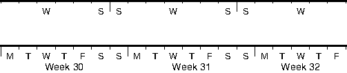
4.4.7 Timestamps on plots: The -U option
4.4.8 Verbose feedback: The -V option
4.4.9 Plot positioning and layout: The -X-Y options
4.4.10 Binary table i/o: The -b option
4.4.11 Number of Copies: The -c option
4.4.12 Data type selection: The -f option
4.4.13 Data gap detection: The -g option
4.4.14 Multiple segment data: The -m option
4.4.15 Lat/Lon or Lon/Lat?: The -: option
4.5 Command line history
4.6 Usage messages, syntax- and general error messages
4.7 Standard input or file, header records
4.8 Verbose operation
4.9 Program output
4.10 Input data formats
4.11 Output data formats
4.12 PostScript features
4.13 Specifying pen attributes
4.14 Specifying area fill attributes
4.15 Color palette tables
4.15.1 Categorical CPT files
4.15.2 Regular CPT files
4.16 Character escape sequences
4.17 Grid file format specifications
4.18 Options for COARDS-compliant netCDF files
4.19 The NaN data value
4.20 GMT environment parameters
5 GMT Coordinate Transformations
5.1 Cartesian transformations
5.1.1 Cartesian linear transformation (-Jx-JX)
5.1.2 Cartesian logarithmic projection
5.1.3 Cartesian power projection
5.2 Linear projection with polar
()
coordinates (-Jp -JP)
6 GMT Map Projections
6.1 Conic projections
6.1.1 Albers conic equal-area projection (-Jb-JB)
6.1.2 Equidistant conic projection (-Jd-JD)
6.1.3 Lambert conic conformal projection (-Jl-JL)
6.1.4 (American) polyconic projection (-Jpoly-JPoly
6.2 Azimuthal projections
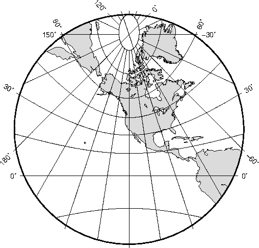
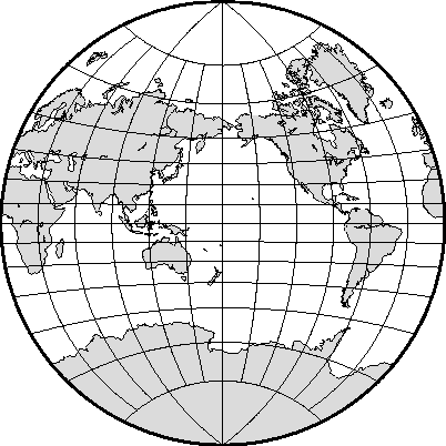
6.2.1 Lambert Azimuthal Equal-Area (-Ja-JA)
6.2.2 Stereographic Equal-Angle projection (-Js-JS)
6.2.3 Perspective projection (-Jg-JG)
6.2.4 Orthographic projection (-Jg-JG)
6.2.5 Azimuthal Equidistant projection (-Je-JE)
6.2.6 Gnomonic projection (-Jf-JF)
6.3 Cylindrical projections
6.3.1 Mercator projection (-Jm-JM)
6.3.2 Transverse Mercator projection (-Jt-JT)
6.3.3 Universal Transverse Mercator (UTM) projection (-Ju-JU)
6.3.4 Oblique Mercator projection (-Jo-JO)
6.3.5 Cassini cylindrical projection (-Jc-JC)
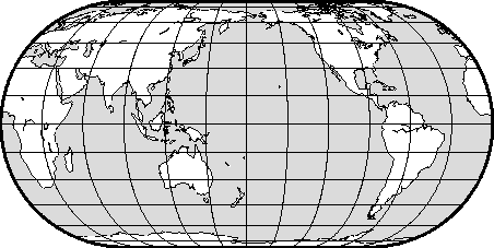
6.3.6 Cylindrical equidistant projection (-Jq-JQ)
6.3.7 Cylindrical equal-area projections (-Jy-JY)
6.3.8 Miller Cylindrical projection (-Jj-JJ)
6.3.9 Cylindrical stereographic projections (-Jcyl_stere-JCyl_stere)
6.4 Miscellaneous projections
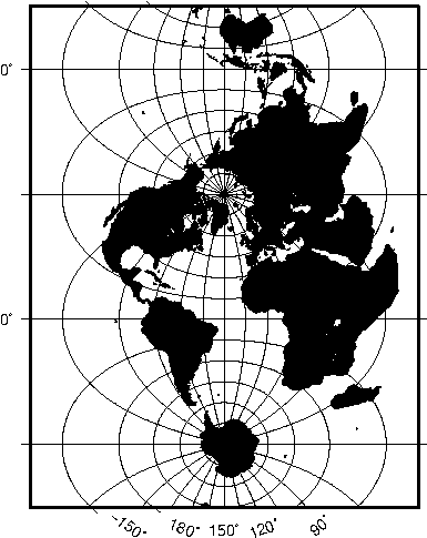
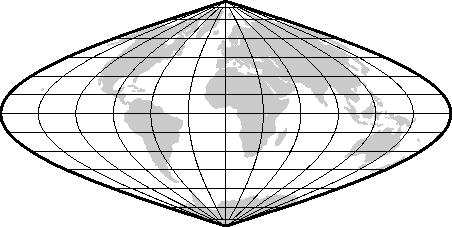
6.4.1 Hammer projection (-Jh-JH)
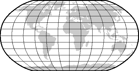
6.4.2 Mollweide projection (-Jw-JW)
6.4.3 Winkel Tripel projection (-Jr-JR)
6.4.4 Robinson projection (-Jn-JN)
6.4.5 Eckert IV and VI projection (-Jk-JK)
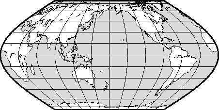
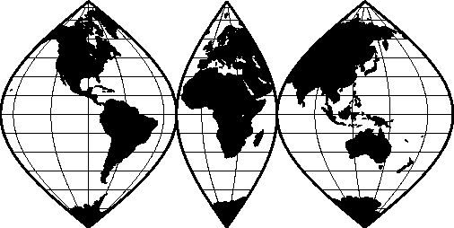
6.4.6 Sinusoidal projection (-Ji-JI)
6.4.7 Van der Grinten projection (-Jv-JV)
7 Creating GMT Graphics
7.1 The making of contour maps
7.2 Image presentations
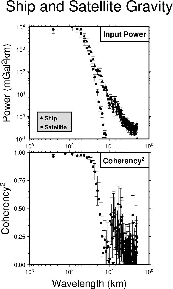
7.3 Spectral estimation and xy-plots
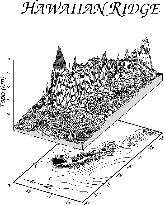
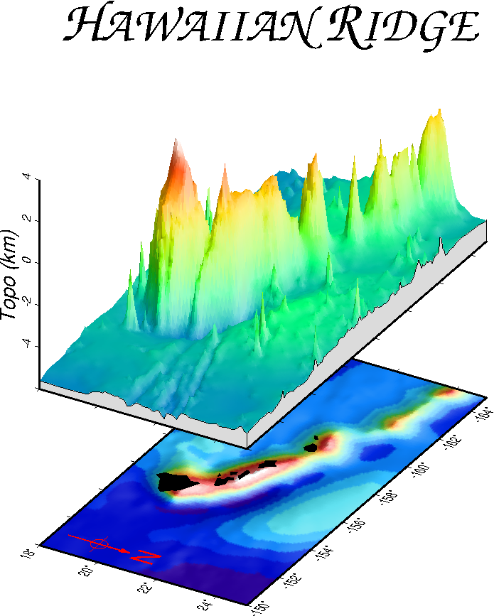
7.4 A 3-D perspective mesh plot
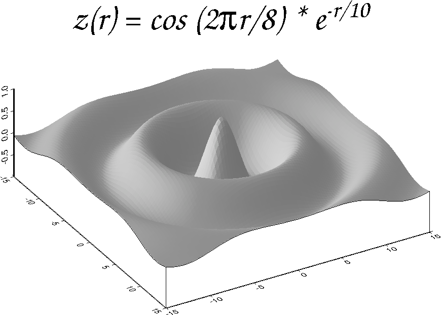
7.5 A 3-D illuminated surface in black and white
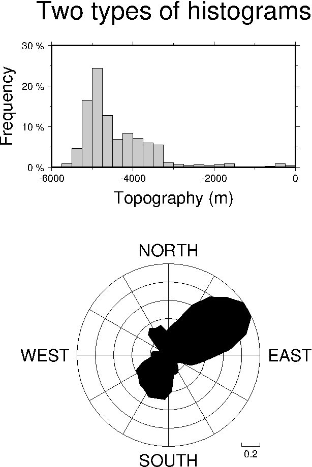
7.6 Plotting of histograms
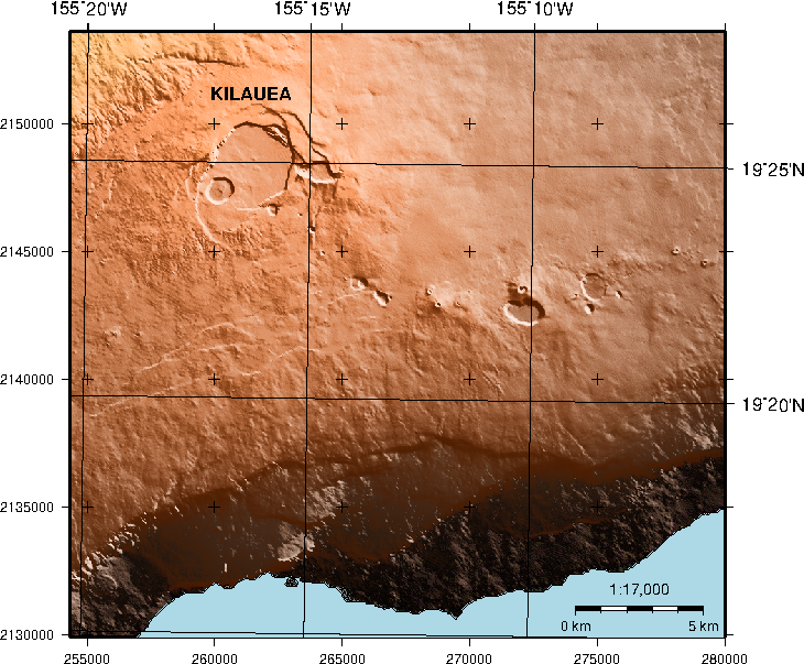
7.7 A simple location map
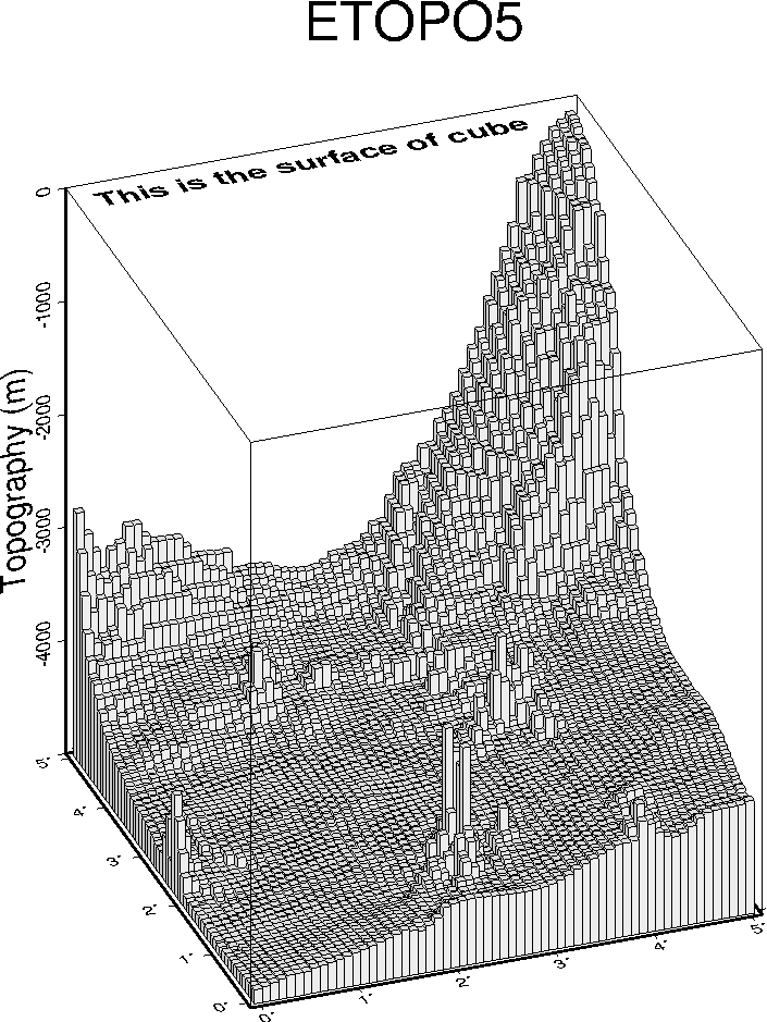
7.8 A 3-D histogram
7.9 Plotting time-series along tracks
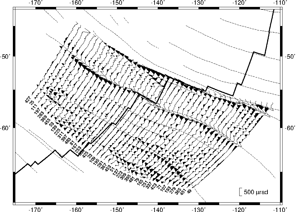
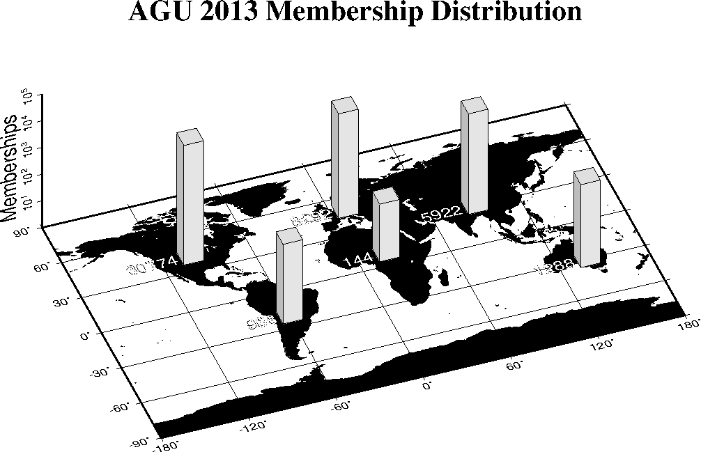
7.10 A geographical bar graph plot
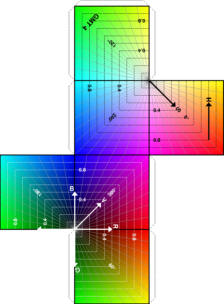
7.11 Making a 3-D RGB color cube
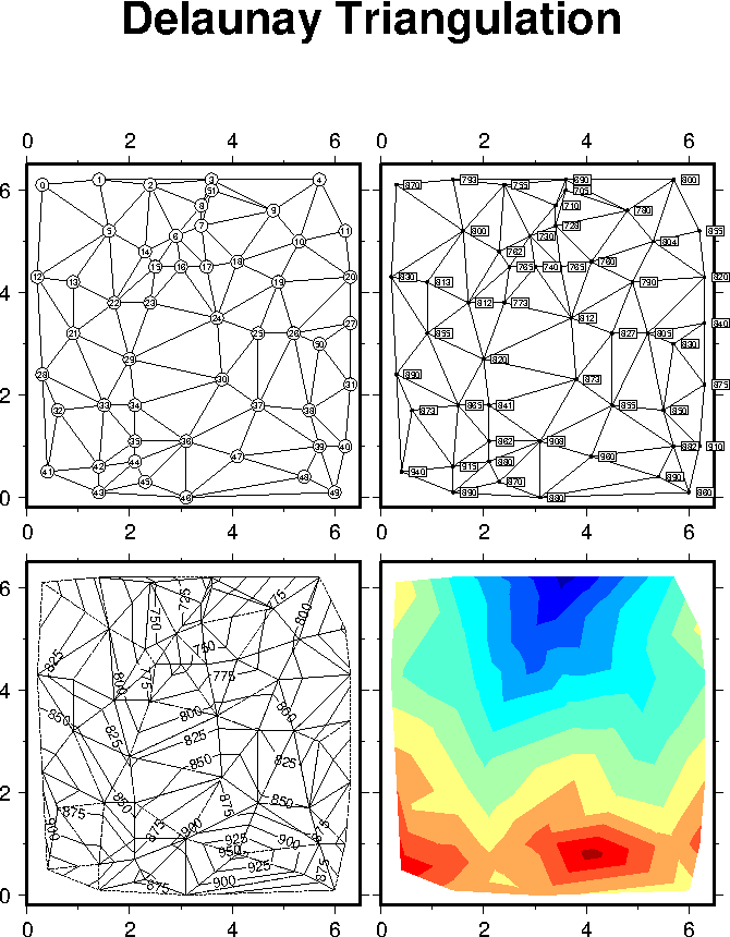
7.12 Optimal triangulation of data
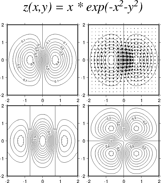
7.13 Plotting of vector fields
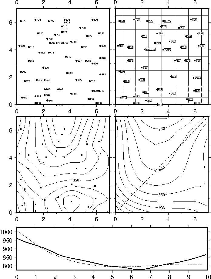
7.14 Gridding of data and trend surfaces
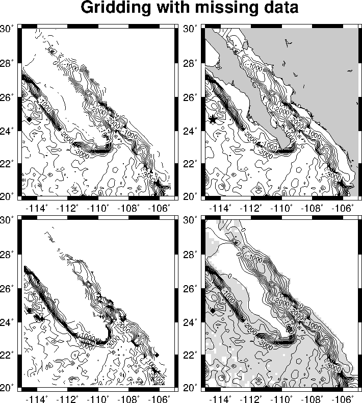
7.15 Gridding, contouring, and masking of unconstrained areas
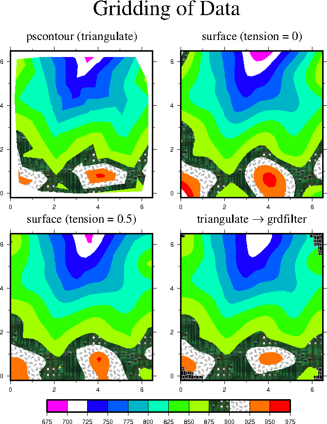
7.16 Gridding of data, continued
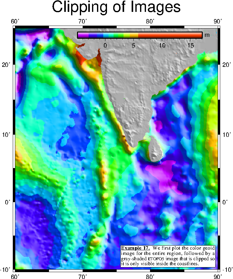
7.17 Images clipped by coastlines
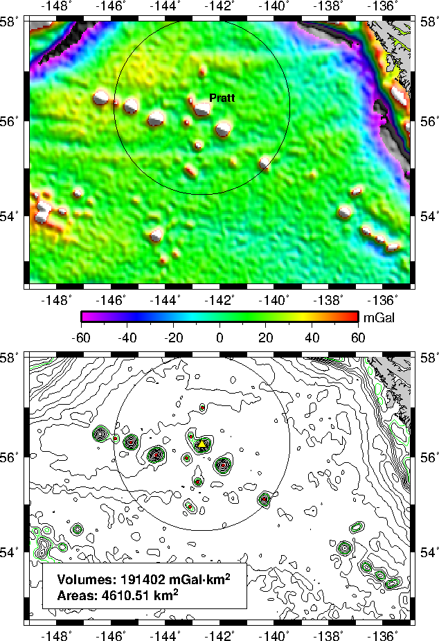
7.18 Volumes and Spatial Selections
7.19 Color patterns on maps
7.20 Custom plot symbols
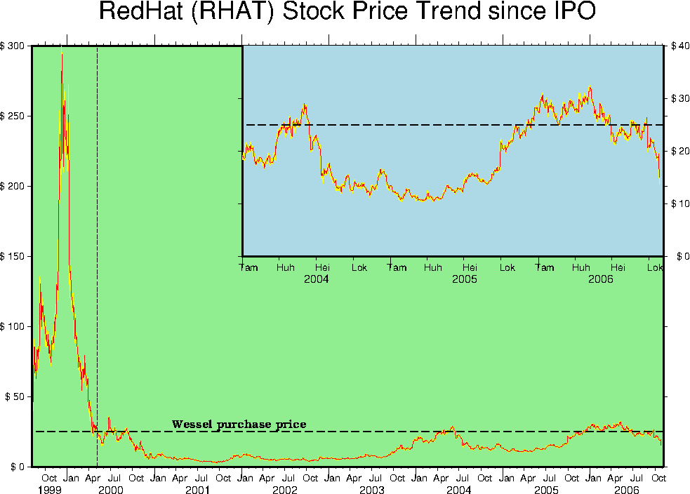
7.21 Time-series of RedHat stock price
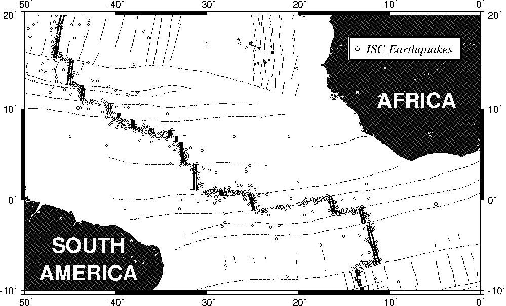
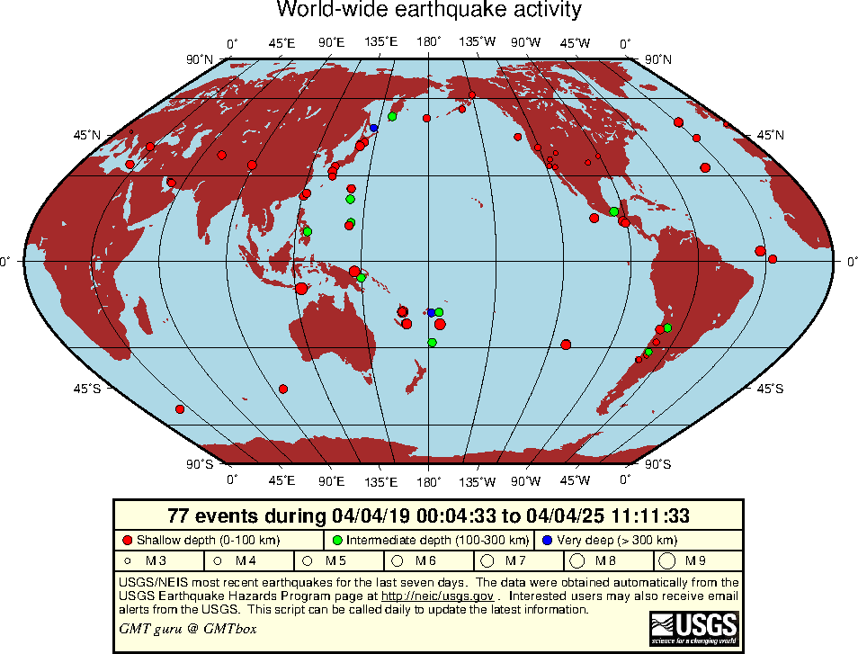
7.22 World-wide seismicity the last 7 days
7.23 All great-circle paths lead to Rome
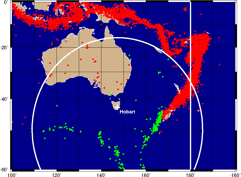
7.24 Data selection based on geospatial criteria
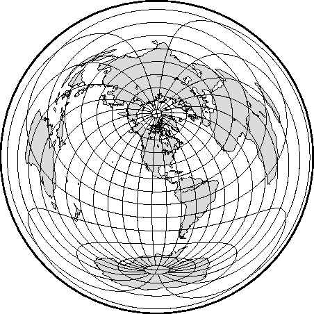
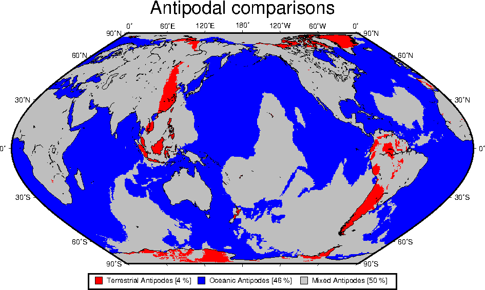
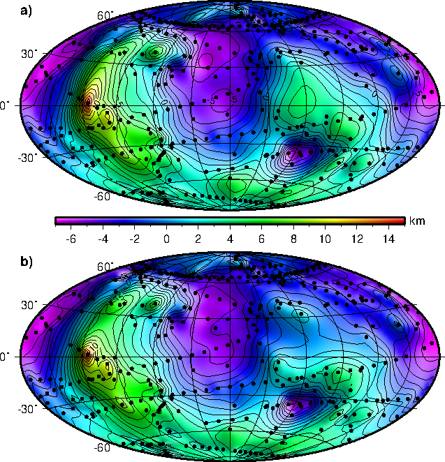
7.25 Global distribution of antipodes
7.26 General vertical perspective projection
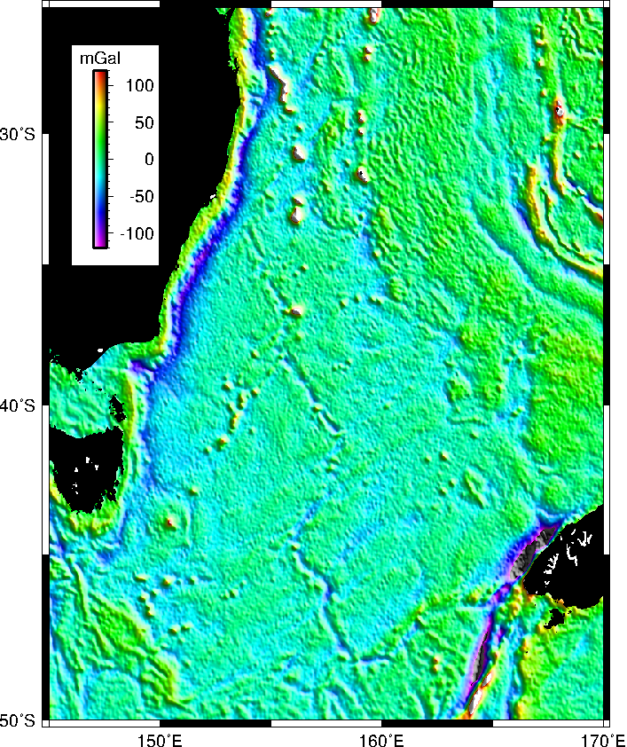
7.27 Plotting Sandwell/Smith Mercator img grids
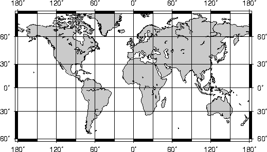
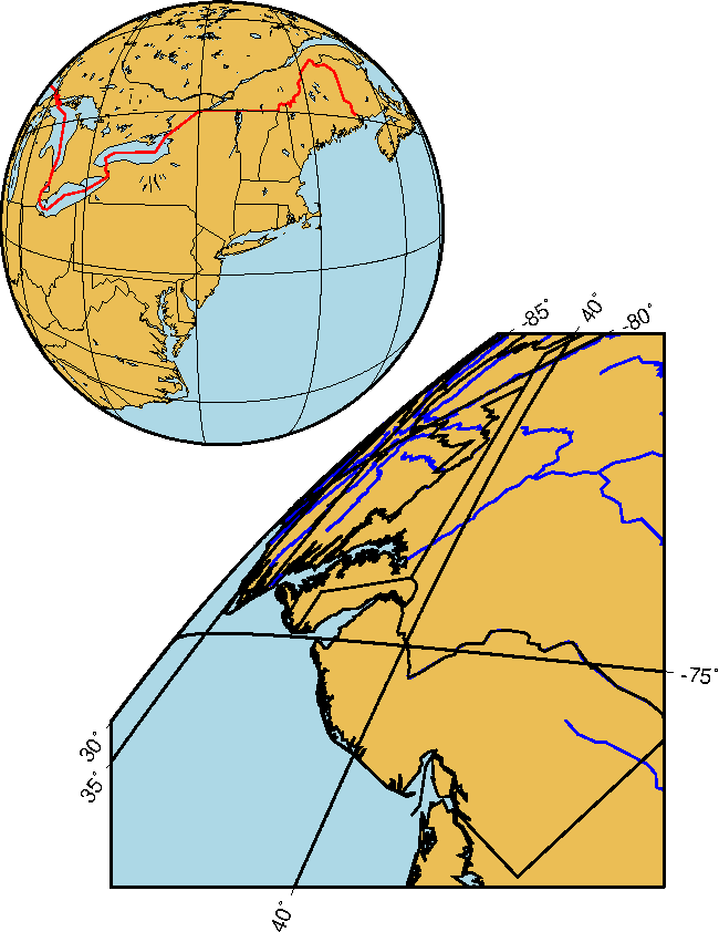
7.28 Mixing UTM and geographic data sets
7.29 Gridding spherical surface data using splines
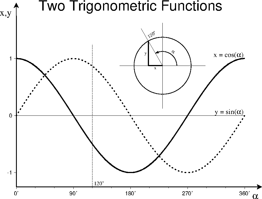
7.30 Trigonometric functions plotted in graph mode
8 Creating GMT Animations
8.1 Animation of the sine function
8.2 Examining DEMs using variable illumination
8.3 Orbiting a static map
8.4 Flying over topography
9 Mailing lists, updates, and bug reports
A GMT supplemental packages
A.1 dbase: gridded data extractor
A.2 gshhg: GSHHG data extractor
A.3 imgsrc: gridded altimetry extractor
A.4 meca: seismology and geodesy symbols
A.5 mex: Matlab/Octave–GMT interface
A.6 mgd77: MGD77 extractor and plotting tools
A.7 mgg: GMT-MGD77 extractor and plotting tools
A.8 misc: Miscellaneous tools
A.9 segyprogs: plotting SEGY seismic data
A.10 sph: spherical triangulation and gridding
A.11 spotter: backtracking and hotspotting
A.12 x2sys: track crossover error estimation
A.13 x_system: track crossover error estimation
A.14 xgrid: visual editor for grid files
B GMT file formats
B.1 Table data
B.1.1 ASCII tables
B.1.2 Binary tables
B.1.3 NetCDF tables
B.2 Grid files
B.2.1 NetCDF files
B.2.2 Gridline and Pixel node registration
B.2.3 Boundary Conditions for operations on grids
B.2.4 Native binary grid files
B.3 Sun raster files
C Including GMT graphics into your documents
C.1 Making GMT Encapsulated PostScript Files
C.2 Converting GMT PostScript to PDF or raster images
C.2.1 When converting or viewing PostScript goes awry
C.2.2 Using ps2raster
C.3 Examples
C.3.1 GMT graphics in LATEX
C.3.2 GMT graphics in PowerPoint
C.4 Concluding remarks
D Availability of GMT and related code
D.1 Source distribution
D.2 Pre-compiled Executables
E Predefined bit and hachure patterns in GMT
F Chart of octal codes for characters
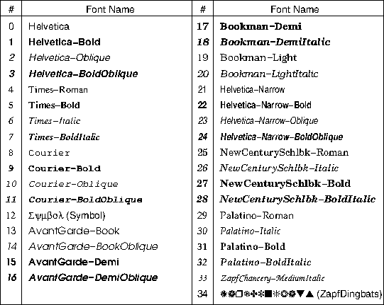
G PostScript fonts used by GMT
H Problems with display of GMT PostScript
H.1 PostScript driver bugs
H.2 Resolution and dots per inch
H.3 European characters
H.4 Hints
I Color Space: The final frontier
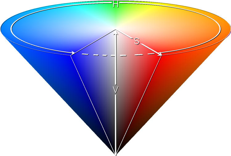
I.1 RGB color system
I.2 HSV color system
I.3 The color cube
I.4 Color interpolation
I.5 Artificial illumination
I.6 Thinking in RGB or HSV
I.7 CMYK color system
J Filtering of data in GMT
K The GMT High-Resolution Coastline Data
K.1 Selecting the right data
K.2 Format required by GMT
K.3 The long and winding road
K.4 The Five Resolutions
K.4.1 The crude resolution (-Dc)
K.4.2 The low resolution (-Dl)
K.4.3 The intermediate resolution (-Di)
K.4.4 The high resolution (-Dh)
K.4.5 The full resolution (-Df)
L GMT on non-UNIX platforms
L.1 Introduction
L.2 Cygwin and GMT
L.3 SFU and GMT
L.4 DJGPP and GMT
L.5 WIN32 and GMT
L.6 OS/2 and GMT
L.7 Mac OS and GMT
M Of colors and color legends
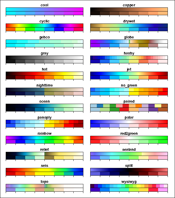
M.1 Built-in color palette tables
M.2 Labeled and non-equidistant color legends
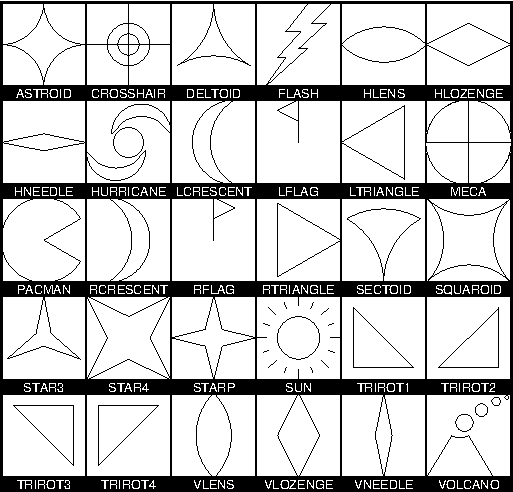
N Custom Plot Symbols
O Annotation of Contours and “Quoted Lines”
O.1 Label Placement
O.2 Label Attributes
O.3 Examples of Contour Label Placement
O.3.1 Equidistant labels
O.3.2 Fixed number of labels
O.3.3 Prescribed label placements
O.3.4 Label placement at simple line intersections
O.3.5 Label placement at general line intersections
O.4 Examples of Label Attributes
O.4.1 Label placement by along-track distances, 1
O.4.2 Label placement by along-track distances, 2
O.4.3 Using a different data set for labels
O.5 Putting it all together
P Special Operations
P.1 Running GMT in isolation mode
P.2 Using both GMT 3 and 4
List of Tables
List of Figures
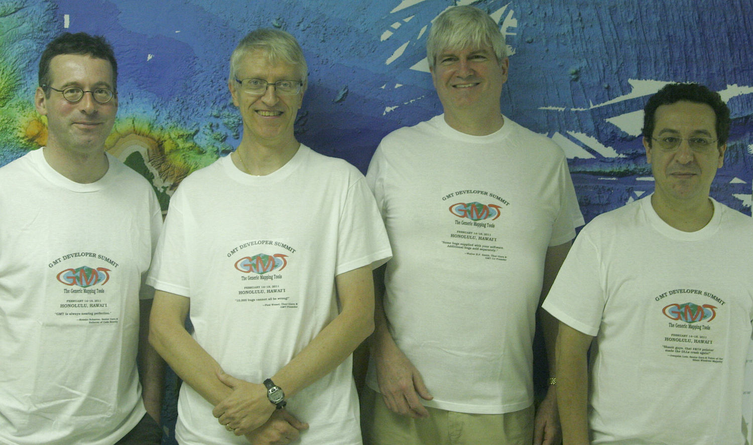
1 The four horsemen of the GMT apocalypse: Remko Scharroo, Paul Wessel, Walter
H.F. Smith, and Joaquim Luis at the GMT Developer Summit in Honolulu, Hawaii during
February 14–18, 2011.4.1 Some GMT parameters that affect plot appearance.4.2 More
GMT parameters that affect plot appearance.4.3 Even more GMT parameters that affect
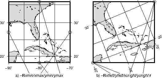
plot appearance.4.4 The plot region can be specified in two different ways. (a) Extreme
values for each dimension, or (b) coordinates of lower left and upper right corners.4.5 The
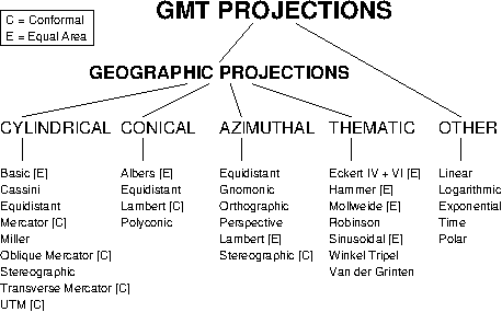
30+ map projections and coordinate transformations available in GMT.4.6 Geographic
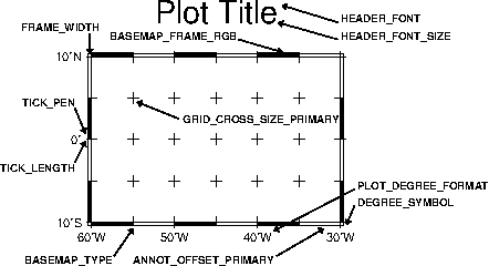
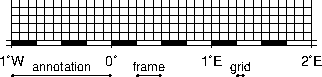
map border using separate selections for annotation, frame, and grid intervals. Formatting
of the annotation is controlled by the parameter PLOT_DEGREE_FORMAT in your
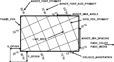
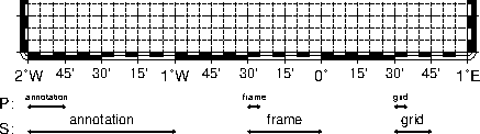
.gmtdefaults4 file.4.7 Geographic map border with both primary (P) and secondary (S)
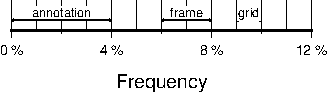
components.4.8 Linear Cartesian projection axis. Long tickmarks accompany annotations,
shorter ticks indicate frame interval. The axis label is optional. We used -R0/12/0/1 -JX3/0.4
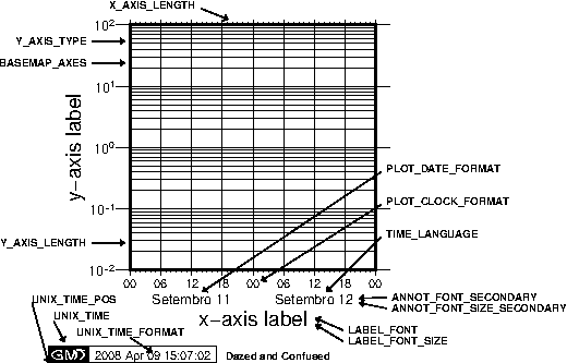
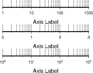
-Ba4f2g1:Frequency::,%:.4.9 Logarithmic projection axis using separate values for annotation,
frame, and grid intervals. (top) Here, we have chosen to annotate the actual values. Interval = 1
means every whole power of 10, 2 means 1, 2, 5 times powers of 10, and 3 means every 0.1 times
powers of 10. We used -R1/1000/0/1 -JX3l/0.4 -Ba1f2g3. (middle) Here, we have chosen to
annotate log
of the actual values, with -Ba1f2g3l. (bottom) We annotate every power of 10 using
log
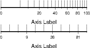
of the actual values as exponents, with -Ba1f2g3p.4.10 Exponential
or power projection axis. (top) Using an exponent of 0.5 yields a
axis. Here,
intervals refer to actual data values, in -R0/100/0/1 -JX3p0.5/0.4 -Ba20f10g5. (bottom)
Here, intervals refer to projected values, although the annotation uses the corresponding
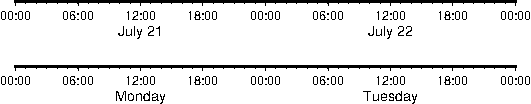
unprojected values, as in -Ba3f2g1p.4.11 Cartesian time axis, example 1.4.12 Cartesian
time axis, example 2.4.13 Cartesian time axis, example 3.4.14 Cartesian time axis, example
4.4.15 Cartesian time axis, example 5.4.16 Cartesian time axis, example 6.4.17 Cartesian
time axis, example 7.4.18 Users can specify Landscape [Default] or Portrait (-P)
orientation.4.19 A final PostScript file consists of any number of individual pieces.4.20 The
-U option makes it easy to “date” a plot.4.21 Plot origin can be translated freely with -X
-Y.5.1 Linear transformation of Cartesian coordinates.5.2 Linear transformation of map
coordinates.5.3 Linear transformation of calendar coordinates.5.4 Logarithmic transformation of
-coordinates.5.5 Exponential
or power transformation of -coordinates.5.6 Polar
(Cylindrical) transformation of ()
coordinates.6.1 Albers equal-area conic map projection6.2 Equidistant conic map
projection6.3 Lambert conformal conic map projection6.4 (American) polyconic
projection6.5 Rectangular map using the Lambert azimuthal equal-area projection.6.6 Hemisphere
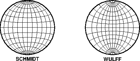
map using the Lambert azimuthal equal-area projection.6.7 Equal-Area (Schmidt) and
Equal-Angle (Wulff) stereo nets.6.8 Polar stereographic conformal projection.6.9 Polar
stereographic conformal projection with rectangular borders.6.10 General stereographic
conformal projection with rectangular borders.6.11 View from the Space Shuttle in Perspective
projection.6.12 Hemisphere map using the Orthographic projection.6.13 World map using
the equidistant azimuthal projection.6.14 Gnomonic azimuthal projection.6.15 Simple
Mercator map.6.16 Rectangular Transverse Mercator map.6.17 A global transverse Mercator
map.6.18 Universal Transverse Mercator zone layout.6.19 Oblique Mercator map using -Joc.
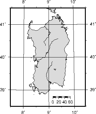
We make it clear which direction is North by adding a star rose with the -T option.6.20 Cassini
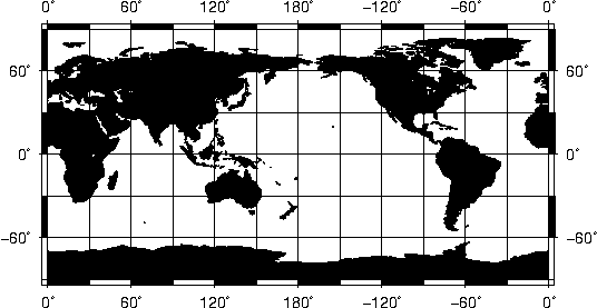
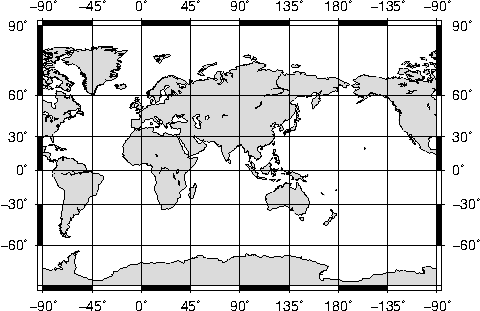
map over Sardinia.6.21 World map using the Plate Carrée projection.6.22 World map using
the Behrman cylindrical equal-area projection.6.23 World map using the Miller cylindrical
projection.6.24 World map using Gall’s stereographic projection.6.25 World map using the
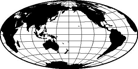
Hammer projection.6.26 World map using the Mollweide projection.6.27 World map using
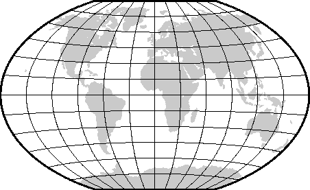
the Winkel Tripel projection.6.28 World map using the Robinson projection.6.29 World map
using the Eckert IV projection.6.30 World map using the Eckert VI projection.6.31 World
map using the Sinusoidal projection.6.32 World map using the Interrupted Sinusoidal
projection.6.33 World map using the Van der Grinten projection.7.1 Contour maps
of gridded data.7.2 Color images from gridded data.7.3 Spectral estimation and
-plots.7.4 3-D
perspective mesh plot (left) and colored version (right).7.5 3-D illuminated surface.7.6 Two kinds
of histograms.7.7 A typical location map.7.8 A 3-D histogram.7.9 Time-series as “wiggles” along
a track.7.10 Geographical bar graph.7.11 The RGB color cube.7.12 Optimal triangulation of
data.7.13 Display of vector fields in GMT.7.14 Gridding of data and trend surfaces.7.15 Gridding,
contouring, and masking of data.7.16 More ways to grid data.7.17 Clipping of images using
coastlines.7.18 Volumes and geo-spatial selections.7.19 Using color patterns and additional
PostScript material in illustrations.7.20 Using custom symbols in GMT.7.21 Time-series of
RedHat stock price since IPO.7.22 World-wide seismicity the last 7 days.7.23 All great-circle
paths lead to Rome.7.24 Data selection based on geospatial criteria.7.25 Global distribution
of antipodes.7.26 General vertical perspective projection.7.27 Plotting Sandwell/Smith
Mercator img grids.7.28 Mixing UTM and geographic data sets requires knowledge of the
map region domain in both UTM and lon/lat coordinates and consistent use of the same map
scale.7.29 Gridding of spherical surface data using Green’s function splines.7.30 Trigonometric
functions plotted in graph mode.8.1 Animation of a simple sine function.8.2 Animation of a DEM
using variable illumination.8.3 Orbiting a static map.8.4 Flying over topography.B.1 Gridline
registration of data nodes.B.2 Pixel registration of data nodes.C.1 Examples of rendered
images in a PowerPoint presentation.C.2 PowerPoint’s “Format Picture” dialogue to set
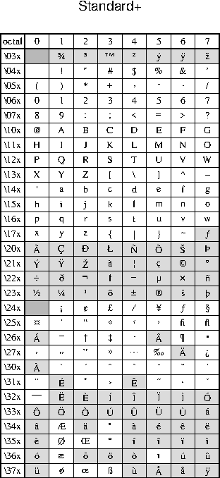
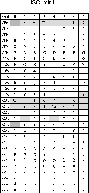
scale and rotation.F.1 Octal codes and corresponding symbols for StandardEncoding (left)
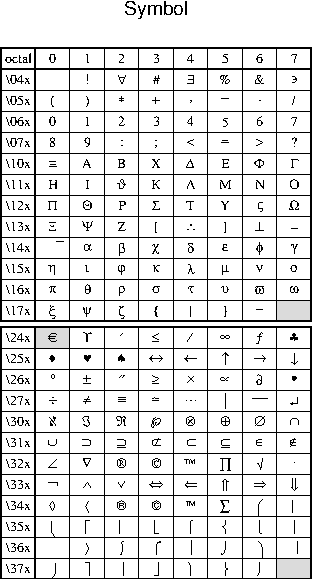
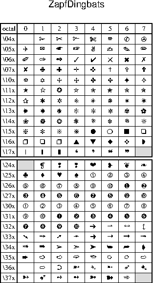
and ISOLatin1Encoding (right) fonts.F.2 Octal codes and corresponding symbols for Symbol
(left) and ZapfDingbats (right) fonts.G.1 The standard 35 PostScript fonts recognized by
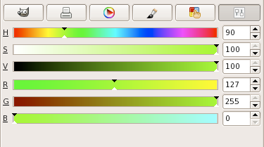
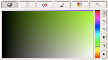
GMT.I.1 Chartreuse in GIMP. (a) Sliders indicate how the color is altered when changing
the H, S, V, R, G, or B levels. (b) For a constant hue (here 90°) value increases to the right and
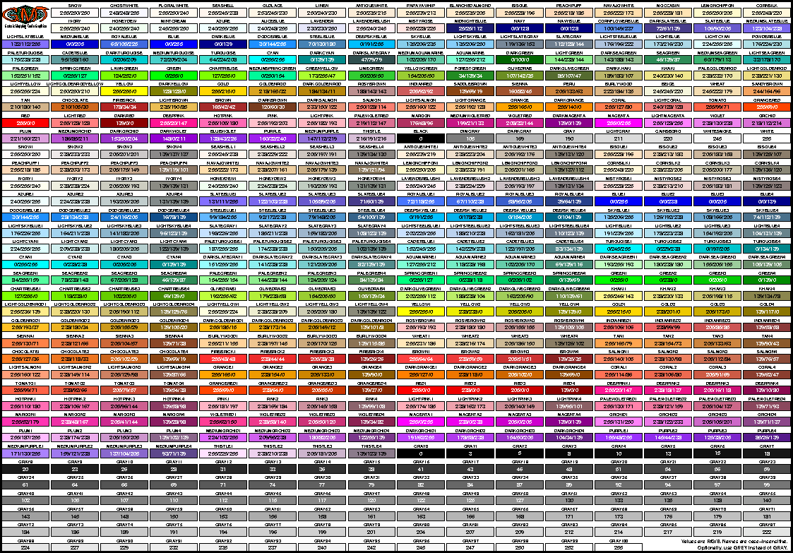
saturation increases up, so the “pure” color is on the top right.I.2 The 555 unique color names
that can be used in GMT. Lower, upper, or mixed case, as well as the british spelling of “grey”
are allowed. A4, Letter, and Tabloid sized versions of this RGB chart can be found in the GMT
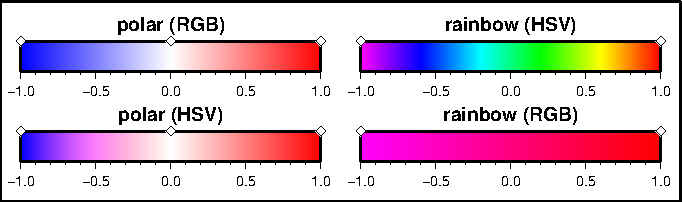
documentation directory.I.3 The HSV color space.I.4 When interpolating colors, the color
system matters. The polar palette on the left needs to be interpolated in RGB, otherwise hue
will change between blue (240°) and white (0°). The rainbow palette should be interpolated in
HSV, since only hue should change between magenta (300°) and red (0°). Diamonds indicate
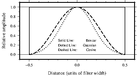
which colors are defined in the palettes; they are fixed, the rest is interpolated.J.1 Impulse
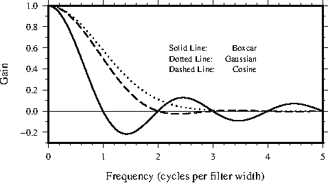
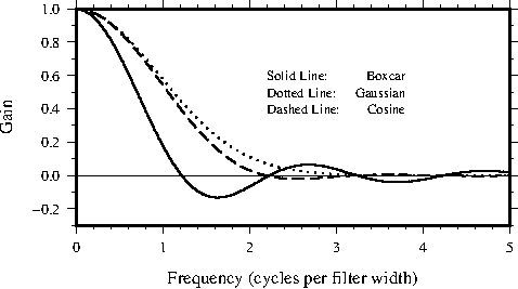
responses for GMT filters.J.2 Transfer functions for 1-D GMT filters.J.3 Transfer functions
for 2-D (radial) GMT filters.K.1 Map using the crude resolution coastline data.K.2 Map
using the low resolution coastline data.K.3 Map using the intermediate resolution coastline
data. We have added a compass rose just because we have the power to do so.K.4 Map using
the high resolution coastline data.K.5 Map using the full resolution coastline data.M.1 The
standard 22 cpt files supported by GMT.M.2 The many forms of color legends created by
psscale.N.1 Custom plot symbols supported by GMT.O.1 Equidistant contour label
placement with -Gd, the only algorithm available in previous GMT versions.O.2 Placing one
label per contour that exceed 1 inch in length, centered on the segment with -Gn.O.3 Four
labels are positioned on the points along the contours that are closest to the locations given in
the file fix.d in the -Gf option.O.4 Labels are placed at the intersections between contours
and the great circle specified in the -GL option.O.5 Labels are placed at the intersections
between contours and the multi-segment lines specified in the -GX option.O.6 Labels
attributes are controlled with the arguments to the -Sq option.O.7 Another label attribute
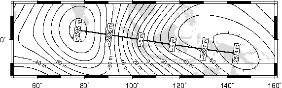
example.O.8 Labels based on another data set (here bathymetry) while the placement is based
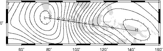
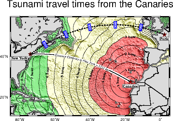
on distances.O.9 Tsunami travel times from the Canary Islands to places in the Atlantic, in
particular New York. Should a catastrophic landslide occur it is possible that New York will
experience a large tsunami about 8 hours after the event.P.1 Example created in isolation mode
Acknowledgments
The Generic Mapping Tools (GMT) could not have been designed without the generous support of several people.
We gratefully acknowledge A. B. Watts and the late W. F. Haxby for supporting our efforts on the original version
1.0 while we were their graduate students at Lamont-Doherty Earth Observatory. Doug Shearer and Roger Davis
patiently answered many questions over e-mail. The subroutine gauss was written and supplied by Bill Menke.
Further development of versions 2.0–2.1 at SOEST would not have been possible without the support from the
HIGP/SOEST Post-Doctoral Fellowship program to Paul Wessel. Walter H. F. Smith gratefully acknowledges
the generous support of the C. H. and I. M. Green Foundation for Earth Sciences at the Institute of
Geophysics and Planetary Physics, Scripps Institution of Oceanography, University of California at San
Diego. GMT series 3.x, 4.x, and 5.x owe their existence to grants EAR-93-02272, OCE-95-29431,
OCE-00-82552, OCE-04-52126, and OCE-1029874 from the National Science Foundation, which we gratefully
acknowledge.
We would also like to acknowledge the feedback we have received from many of the users of earlier versions.
Many of these suggestions have been implemented, and the bug reports have been useful in providing more robust
programs. Specifically, we would like to thank Michael Barck, Manfred Brands, Stephan Eickschen, Ben
Horner-Johnson, John Kuhn, Angel Li, John Lillibridge, Andrew Macrae, Alex Madon, Greg Neumann, Lloyd
Parkes, Ameet Raval, Georg Schwarz, Richard Signell, Peter Schimidt, Dirk Stoecker, Eduardo Suárez, Mikhail
Tchernychev, Malte Thoma, David Townsend, Garry Vaughan, William Weibel, Florian Wobbe, and many
others, including their advice on how to make GMT portable to a wide range of platforms. John
Lillibridge provided the original example 11; Hanno von Lom helped resolve early problems with DLL
libraries for Win32; Lloyd Parkes enabled indexed color images in PostScript; Kurt Schwehr maintains
the Fink packages; Wayne Wilson implemented the full general perspective projection; and William
Yip helped translate GMT to POSIX ANSI C and incorporate netCDF 3. The SOEST RCF staff
(Ross Ishida, Pat Townsend, and Sharon Stahl) provided valuable help on Linux, web, and CGI script
issues.
Honolulu, HI, College Park, MD, Cornish, NH, and Faro, Portugal, July 2018
The GMT Documentation Project
Starting with GMT version 3.2, all GMT documentation was converted from Microsoft Word to LATEX files.
This step was taken for a number of reasons:
- Having all the documentation source available in ASCII format makes it easier to access by several
GMT developers working on different platforms in different countries.
- GMT scripts can now be included directly into the text so that the documentation is automatically
up-to-date when scripts are modified.
- All figures are generated on the fly and included as GMT EPS files which thus are always up-to-date.
- It is easy to convert the LATEX files to other formats, such as HTML, SGML, PostScript, and PDF.
- The whole task of assembling the pieces, be it generating figures or extracting text portions from the
master archive under subversion control, is automated by a makefile.
- Only free software are used to maintain the GMT Documentation.
Please post a New Issue from GMT home page if you find errors or inconsistencies in the documentation.
A Reminder
If you feel it is appropriate, you may consider paying us back by citing our EOS articles on GMT (and perhaps
also our Geophysics article on the GMT program surface) when you publish papers containing results or
illustrations obtained using GMT. The EOS articles on GMT are
- Wessel, P., and W. H. F. Smith, New, improved version of Generic Mapping Tools released, EOS Trans.
Amer. Geophys. U., vol. 79 (47), pp. 579, 1998.
- Wessel, P., and W. H. F. Smith, New version of the Generic Mapping Tools released, EOS Trans. Amer.
Geophys. U., vol. 76 (33), pp. 329, 1995.
- Wessel, P., and W. H. F. Smith, New version of the Generic Mapping Tools released, EOS Trans. Amer.
Geophys. U. electronic supplement, http://www.agu.org/eos_elec/95154e.html, 1995.
- Wessel, P., and W. H. F. Smith, Free software helps map and display data, EOS Trans. Amer. Geophys.
U., vol. 72 (41), pp. 441, 445-446, 1991.
The article in Geophysics on surface is
- Smith, W. H. F., and P. Wessel, Gridding with continuous curvature splines in tension, Geophysics, vol.
55 (3), pp. 293-305, 1990.
GMT includes some code supplied by others, in particular the Triangle code used for Delaunay triangulation.
Its author, Jonathan Shewchuk, says
“If you use Triangle, and especially if you use it to accomplish real work, I would like very much
to hear from you. A short letter or email (to jrs@cs.cmu.edu) describing how you use Triangle will
mean a lot to me. The more people I know are using this program, the more easily I can justify
spending time on improvements and on the three-dimensional successor to Triangle, which in turn
will benefit you.”
A few GMT users take the time to write us letters, telling us of the difference GMT is making in their work.
We appreciate receiving these letters. On days when we wonder why we ever released GMT we pull these letters
out and read them. Seriously, as financial support for GMT depends on how well we can “sell” the idea to funding
agencies and our superiors, letter-writing is one area where GMT users can affect such decisions by supporting the
GMT project.
Copyright and Caveat Emptor!
Copyright ©1991 – 2018 by Paul Wessel and Walter H. F. Smith
The Generic Mapping Tools (GMT) is free software; you can redistribute it and/or modify it under the terms of the
GNU General Public License as published by the Free Software Foundation.
The GMT package is distributed in the hope that it will be useful, but WITHOUT ANY WARRANTY;
without even the implied warranty of MERCHANTABILITY or FITNESS FOR A PARTICULAR PURPOSE. See
the file LICENSE.TXT in the GMT directory or the GNU General Public License for more details.
Permission is granted to make and distribute verbatim copies of this manual provided that the copyright notice
and these paragraphs are preserved on all copies. The GMT package may be included in a bundled distribution of
software for which a reasonable fee may be charged.
The Generic Mapping Tools (GMT) does not come with any warranties, nor is it guaranteed to work on your
computer. The user assumes full responsibility for the use of this system. In particular, the School of Ocean and
Earth Science and Technology, the National Oceanic and Atmospheric Administration, the National Science
Foundation, Paul Wessel, Walter H. F. Smith, or any other individuals involved in the design and maintenance of
GMT are NOT responsible for any damage that may follow from correct or incorrect use of these
programs.
Typographic conventions
In reading this documentation, the following provides a summary of the typographic conventions used in this
document.
- User input and GMT or UNIX commands are indicated by using the typewriter type style, e.g.,
chmod +x job03.sh.
- The names of GMT programs are indicated by the bold, sans serif type style, e.g., we plot text with
pstext.
- The names of other programs are indicated by the bold, slanted type style, e.g., grep.
- File names are indicated by the underline type style, e.g., gmt.h.
Chapter 1
Preface
While GMT has served the map-making and data processing needs of scientists since
1988,
the current global use was heralded by the first official release in EOS Trans. AGU in the fall of 1991. Since
then, GMT has grown to become a standard tool for many users, particularly in the Earth and Ocean
Sciences. Development has at times been rapid, and numerous releases have seen the light of day since
the early versions. For a detailed history of the changes from release to release, see file ChangeLog
in the main GMT directory. For a nightly snapshot of ongoing activity, see the online ChangeLog
page.
The success of GMT is to a large degree due to the input of the user community. In fact, most of the
capabilities and options in GMT programs originated as user requests. We would like to hear from you should you
have any suggestions for future enhancements and modification. Please send your comments to the user forum on
the GMT home page.
1.1 What is new in GMT 4.x?
Since the release of GMT 5.x, GMT 4.x has continued to see corrections of legacy bugs and problems,
but no new features will be added. Therefore, the GMT 4.x releases were mostly bug-fixes as all
development is now focussed on GMT 5; this new series, released Nov-5, 2013, is distinguished by
being completely restructured to allow developers access to high-level GMT modules from a variety
of programming environments. Below is a brief history of the development milestones in the 4.x
series. All work, including bug fixes, has now ceased for the GMT 4 series, making 4.5.18 the final
release.
1.1.1 Overview of GMT 4.5.18 [Jul-1, 2018]
We have corrected one minor bug in this final release of the GMT4 series:
-
gmt_stat.c
- : Fix issue # 1185 in t-critical calculation.
1.1.2 Overview of GMT 4.5.17 [Jan-1, 2018]
We have corrected a few minor bugs and other issues in two of the supplements:
-
pscontour.c
- : Fix issue #1173.
-
meca/psmeca.c
- : Fix issue #1171.
-
mgd77/mgd77.c
- : Fix writing issue for mgd77 header.
-
gmt_support.c
- : PostScriptwrong equations for BC d2z/dxdy for grids. Made tiny changes to ex14
PostScript and grdimage.ps test.
1.1.3 Overview of GMT 4.5.16 [June-25, 2017]
We have corrected a few bugs and other issues for individual programs in the mgd77 supplement:
-
mgd77/mgd77.c
- : Fix format order search. Issue #1039. Set the priority of formats to match GMT5:
MGD77+ first, then MGD77T, MGD77, and plain text table.
-
mgd77/mgd77convert.c
- : Specify new search order if extension not given.
-
mgd77/mgd77header.c
- : Added -Mt and removed unused code. Removed unrelated options from
careless copy/paste via mgd77/mgd77list.c.
-
mgd77/mgd77info.c
- : Specify new search order if extension not given.
-
mgd77/mgd77list.c
- : Clarified usage of E77 bits in source and docs Did not use bitflags set with -Af
correctly.
-
mgd77/mgd77path.c
- : Specify new search order if extension not given.
-
mgd77/mgd77sniffer.c
- : Replace wrong use of common options -B, -K, -P with options -M, -E, and
-Z, respectively.
-
mgd77/mgd77track.c
- : Failed to reduce time by time_inc before plotting marker. Specify new search
order if extension not given.
1.1.4 Overview of GMT 4.5.15 [October-1, 2016]
We fixed some old compiler-flags that prevented compilation under recent version of Solaris and removed some
copyrighted Numerical Recipes code in the meca supplement that were not even used. In addition, we made a few
bug corrections for individual programs:
-
gmt_map.c
- : Did not compute correct length of clip path for azimuth-elevation projection.
-
pscontour.c
- : Would crash if no contours were requested.
-
grdtrack.c
- : The -Z option did not deactivate -: for output.
-
surface.c
- : Critical bug in which the test to determine if a Cartesian data point is “close” to a node would
find most points to be close and bypass the Briggs scheme.
-
mgd77/mgd77list.c
- : Can only use logical field tests on observed data columns.
-
sph/sphinterpolate.c
- : Fix the vertical flipping under -Q0 mode.
1.1.5 Overview of GMT 4.5.14 [Nov-1, 2015]
Another bug-fix release with a few bug corrections for individual programs:
-
gmt_plot.c
- : Fix issue # 662 with graph arrows for negative scales. Flipping the n/s sides array when lon
and -y axes fixes issue #520.
-
gmt_support.c
- : Fix bug in jump near Dateline in gmt_inonout_sphpol_count, affecting
inside/outside spherical cases, reported in message-2219.
-
meca/psmeca.c
- : Was unable to read any value x and y coordinates.
-
share/cpt/GMT_wysiwyg.cpt
- : Fix typo in blue for high end [Issue #689].
1.1.6 Overview of GMT 4.5.13 [Jan-1, 2015]
Another bug-fix release. The default coastline version is now at 2.3.4. Below is the list of bug corrections for
individual programs:
-
gmt_bcr.c
- : Fixed problem with points slightly outside region causing an access violation; see issue #620.
-
gmt_map.c
- : The map region clip path for -JE/-Je was hardwired to a full circle and did not care about
-R setting. When -R...r and -JE/-Je was given the search for enclosing geographic boundaries
failed when either the S or N pole was the projection’s antipole. Rect clipping with -Rw/s/e/nr could
introduce stray lines when dataset has features about 180 degrees away from the user’s area. Could run
into trouble clipping polygons for non-periodic maps. Added more checks in GMT_wesn_clip.
-
gmt_plot.c
- : Left a PSL variable undefined when grdimage plotted a grid with x = longitude and y =
Cartesian.
-
gmtmath.c
- : Fix the order of when input files and -C interact.
-
gmtselect.c
- : The -Fpolygon option might miss points because the io-machinery would sometimes set
the min/max longitudes found incorrectly. The -Z option needed to pass records with NaNs.
-
grdfilter.c
- : Fix y-shifts when -I sets smaller output spacing (issue #616).
-
grdmath.c
- : Fix bug in grdmath’s KM2DEG operator.
-
psxy.c
- : Fixed wrap-around issue in fault lines.
-
psxyz.c
- : Fixed wrap-around issue in fault lines.
-
sample1d.c
- : Fix resampling for decreasing t values.
-
mgd77/mgd77sniffer.c
- : Needed to check that grid values used in decimate function also were within
reasonable range.
-
x2sys/x2sys_solve.c
- : Fix problems that arise when a track has less crossovers than model parameters.
1.1.7 Overview of GMT 4.5.12 [Mar-1, 2014]
Unbeknownst to many software developers, Apple changed the behavior of strcpy in Mavericks in an effort to
strengthen the security of user codes. This caused ps2raster.c to crash for OS X users when it in the past had
worked fine. The problem was easily corrected but meant that all those who had just upgraded to
Mavericks were in a bind. This update corrects this problem, as well as several bugs. We also had
to revert the behavior of the grdmath operator SDIST to again return km instead of degrees since
it cannot do degrees for geodesics. By doing km it is now aligned with what PDIST and LDIST
return for geographic data, and matches the behavior in GMT5. Some scripts had to be modified to
handle the new behavior. If you use SDIST you may wish to check your usage. To assist users wanting
spherical degrees we have added the two conversion operators KM2DEG and DEG2KM that can be
used if the ELLIPSOID setting is Sphere. Finally, since GSHHG 2.3.0 has now been released we set
that as the default coastline version. Below is the list of bug corrections for individual library files or
programs:
-
gmt_grdio.c
- : When building the grid command string it could exceed its maximum length if the
argument became exactly the max length of the array; then the final extra zero character would be added
and exceed array length. This was a rare occurrence. Thanks to Joachim Saul for pointing it out.
-
gmt_map.c
- : Protect against longitude wrap in the Haversine and Rudoe formulae for distances. Prevent
integer overflow when calculating image array size.
-
gmt_plot.c
- : Grid crosses clipped by map boundary were badly reoriented.
-
gmt_proj.c
- : GMT_eckert4 and GMT_eckert6 did not increment iteration counter and could in rare
situations get stuck in an infinite loop.
-
gmt_support.c
- : Allow GMT_crossover to deal with global wrapped data.
-
gmt_vector.c
- : Add protection against introduced longitude-jumps produced by resampling in
GMT_fix_up_path.
-
grdlandmask.c
- : Failed to fill in some partial bins with no actual coastlines going through, in particular
when crossing Greenwich.
-
grdmath.c
- : Operator SDIST used spherical calculations for geodesics and ellipsoidal calculations great
circles (we want the opposite). Now returning distances in km.
-
grdvector.c
- : The new testing of -I arguments failed for some grids. Vector direction did not adjust
when negative scales were used in -JX or -Jx.
-
ps2raster.c
- : Did not check if source and destination given to strcpy were the same; this was always
undefined behavior that now triggers an exit. Also added better check on the return code from the
system calls in case gs or gdal_translate return with an error. Finally, make sure that image references
in KML files do not carry a directory name.
-
pscoast.c
- : The processing of -I and -N levels and pens could get out of sync so that the wrong pen
was used for the specified feature.
-
pslib.c
- : Take superscripts and subscripts into account when determining dimensions of text box. Also
auto-widen paragraph width if the widest word actually is wider that chosen paragraph width.
-
psxy.c
- : Vector direction did not adjust when negative scales were used in -JX or -Jx.
-
psxyz.c
- : Vector direction did not adjust when negative scales were used in -JX or -Jx.
-
mgd77/mgd77header.c
- : Fix selection of 10x10 degree identifiers.
-
misc/gmt2kml.c
- : Make sure the default style IDs are unique for each process.
-
x2sys/x2sys.c
- : Mishandled the assignment of segment number for each record.
1.1.8 Overview of GMT 4.5.11 [Nov-5, 2013]
Note: Due to a few technical issues we had an aborted update to 4.5.10 that was briefly released, then retracted;
hence the 4.5.11-numbered version. GMT 4.5.11 is another service release with bug-fixes only. The only non-bug
change was adding the latest dimensions for recent Sandwell/Smith img files that go up to 85°, and adding
definition file dat.def for mgd77 ASCII DAT format to the x2sys supplement. We also had to modify the –S option
in pscontour.c to address a bug. This GMT release also coincides with the latest GSHHG release version 2.2.4
which adds a few missing lakes to California and fixes an error in the Baffin Island coastline and removes
skinny spikes from numerous features. Below is the list of bug corrections for individual library files or
programs:
-
gmt_customio.c
- : The magic recognition of native bit grids failed due to bad math. Wrote wrong number
of bytes per record for odd-width Sun rasterfiles.
-
gmt_grdio.c
- : Would restrict grid region in grdimage.c despite doing a global map with azimuthal
projections.
-
gmt_io.c
- : Formats for degree annotations using colons should never end in a trailing colon. Could
not properly decode yyodd (no delimiter) time coordinates like 12Oct24. The GMT_import_table
function checked for greenwich before assigning the input data.
-
gmt_init.c
- : Shifted JD origin by one day (24 Nov, instead of 25 Nov).
-
gmt_map.c
- : The oblique Mercator would get the pole on the wrong hemisphere. When -Jx is
used with longitudes we must use the wesn clipping and outside functions, not the Cartesian
ones. Fixed clipping problem in GMT_wesn_clip for regions larger than 180 but less than 360.
GMT_grdproject_init did not handle increments that had been specified as units, e.g., -D30e.
-
gmt_plot.c
- : Did not check for map-jumping in GMT_plot_rectangle (psxy -SJ).
-
gmt_proj.c
- : Inverse -JR blew up at origin; now added a check. Needed to allow for minor round-off
when determining if a point is beyond the horizon for -JG general perspective projection.
-
blockmean.c
- : Did not use data near west column nodes that were off by 360 for gridline registered
grids.
-
blockmedian.c
- : Did not use data near west column nodes that were off by 360 for gridline registered
grids.
-
blockmode.c
- : Did not use data near west column nodes that were off by 360 for gridline registered
grids.
-
filter1d.c
- : Susceptible to round-off when determining t of first and last output point when -T was not
given.
-
gmtmath.c
- : The MIN and MAX operators ignored NaNs, but result should be NaN if one of the operands
equal NaN. Wrong index order in rarely used SVD part of LSQFIT.
-
gmtset.c
- : Did not write values to .gmtdefaults4 if BASEMAP_TYPE was graph or inside.
-
grdfft.c
- : Fix normalization for std.dev of power estimate in -E.
-
grdimage.c
- : Fix bug represented by the globalgrid.sh test script for mix of -R selections and
pixel/gridline choices.
-
grdblend.c
- : Despite geographic grids there were no check to shift a grid region by
to match specified output region.
-
grdlandmask.c
- : Did not set output as geographic after using -Jx1d.
-
grdmath.c
- : The MIN and MAX operators ignored NaNs, but result should be NaN if one of the operands
equal NaN. The XOR operator was incorrect, it is now clarified to be 0 if A == NaN and B == NaN,
NaN if B == NaN, else A. Fix bug in CURV operator.
-
grdsample.c
- : When given a -Rg grid and giving -Rg on command line, the output region became
-360/0 instead of the expected 0/360.
-
grdtrend.c
- : We messed up an interior parameter array in the 2009-10-14 fix in 4.5.2. This affected robust
fits and grids with NaNs.
-
grdvector.c
- : Did not reject vectors on far side of orthographic maps. Enforce that -Idx/dy must be
multiples of grid dx/dy and abort if they are not. Before we would crash, hang, etc.
-
greenspline.c
- : The normalization for 2-D with geographic data
suffered from not checking that longitudes may be off by
.
Needed -f in order to select -f0T input, plus it made assumptions about getting lon,lat despite not
being selected. When -T was used the number of z-layers (1) was not initialized.
-
nearneighbor.c
- : Clarify how -N works, what the defaults are, and let the minimum number of sectors
default to 50% of sectors instead of a hard-wired 2.
-
pscontour.c
- : Added -St to skip triangles whose 3 vertices are outside domain; in contrast, -S or -Sp
skips all points outside domain before triangularization.
-
psmask.c
- : Multiple, ancient bugs fixed: properly mark used edges, fix memory allocations, not report
clipping if -D is used, starting point for a contour was not offset by 1/2 pixel. Was off by one in the
grid index calculation.
-
pstext.c
- : The line in -D...v was plotted on top rather than beneath box.
-
xyz2grd.c
- : For -E, must read data as double so can properly compare with the nodata_value read as
double.
-
meca/psvelo.cc
- : Called get_trans at north pole and tried to find a point further north. Did not honor
the -N setting.
-
mgd77/mgd77list.cc
- : The azimuth written was back-azimuth, not forward. Picked id = time_column
when set was 1 (custom), causing the first custom data column to be formatted as time (this is for the
netCDF format files).
-
sph/sphdistance.c
- : Make sure we visit replicated columns for gridline registered grids.
1.1.9 Overview of GMT 4.5.9 [Jan-1, 2013]
Predominantly a bug-fix release, we also have made some changes to GSHHS. First, GSHHS is now called
GSHHG, the “Global Self-consistent Hierarchical High-resolution Geography”, since GSHHG contains both
shorelines as well as political boundaries and rivers. GSHHG, being required by both GMT 4 and 5, is now
released separately from GMT. Second, we have made some minor changes to a few islands that have shown to be
offset with respect to modern data (Tahiti, Moorea, and Mehetia in South Pacific and Agalega Islands in the Indian
Ocean). Third, we have removed the item known as “Sandy Island” in the Corel Sea since available satellite data
show no evidence of land in this area. Finally, we have purged 48 duplicates of very small islands
(mostly in the Red Sea, Persian Gulf, and the Cook-Austral archipelago) where inaccurate WDBII
versions and accurate WVS versions of the same features had survived our initial processing. This
GMT release thus coincides with the latest GSHHG release version 2.2.2. We also fixed a typo in the
MJD date in the gmtdefaults.txt documentation and updated the CM4 coefficient files for the mgd77
supplement.
Below is the list of bug corrections for individual programs:
-
gmt_grdio.c
- : For -R...r the adjusted w/e/s/n for a grid could have excessive e/n values, leading to extra
work and large intermediate grids.
-
gmt_map.c
- : With -R...r and -JE, pscoast could end up trying to paint a block that is outside the
rectangular region yet whose projection completely contains the region. Clipping function could shift
the w/e boundaries by an extra 360, thus finding nothing inside in some pscoast tiles.
-
gmt_shore.c
- : Will now look for either “.nc” or “.cdf” GSHHG files; needed since GSHHG is now
stand-alone. Also look in given dir directory if compiled in via configure with-gshhg-dir=dir.
-
gmt_support.c
- : Improved contour orientation function for grdcontour -F, thanks to Thomas
Hottendorff. Resolved case of crossings at perfect saddles.
-
gmtmath.c
- : Operators UPPER and LOWER did not assign output to rows that contain NaN.
-
grdfilter.c
- : For -D4 we must set scale based on max |lat| in input grid.
-
grdproject.c
- : The north coordinate would get reset to 2 when -C was used, thus creating wrong map
setup calls.
-
project.c
- : Had to backport changes implemented in GMT 5 to make the -C-T-G combination work
properly.
-
pslib.c
- : Typo in array index in European letter shorthands for German double-s; thanks to David
Lachapelle.
-
psxy.c
- : Would hang for -Jx...d due to wrong meter-per-degree variable.
-
meca/psvelo.c
- : Bug in parsing the -A arguments.
-
mgd77/mgd77.c
- : Copied 4 rather than 2 characters into day field, causing overflow and SEGV.
-
mgd77/mgd77magerf.c
- : The -A+ttime option did not parse ISO calendar items.
-
misc/dimfilter.c
- : Initialized a max value to -DBL_MIN instead of -DBL_MAX.
-
spotter/backtracker.c
- : First and last point in a path was not converted back from geocentric
coordinates.
-
spotter/libspotter.c
- : Did not check for time reversals among total reconstruction rotations.
-
spotter/originator.c
- : Bad format statement would wreck the 5th output column when run in default
mode.
-
x2sys/x2sys_cross.c
- : Did not convert time to seconds before calculating speed. Disallowed the
distance gap check if time was present.
1.1.10 Overview of GMT 4.5.8 [Apr-1, 2012]
Another bug-fix release, except for the mgd77 supplement where we now have added support for the new
MGD77T tab-delimited format introduced by NGDC, and for ps2raster.c under Windows where the
Ghostscript executable path is now fetched from the registry. In case that fails, we fall back to the old “get it
from the path” mechanism. One common bug shared by several programs was the failure to consult
FIELD_DELIMITER and/or D_FORMAT for ASCII output formatting. Below is the list of bug corrections for
individual programs:
-
gmt_customio.c
- : Change nx and ny to “unsigned short int” type in surfer6 header. Note that original
format specification by Golden Software clearly say they are “short int” but this change shouldn’t break
anything and will allow dealing with larger grid sizes.
-
gmt_grdio.c
- : The opening of files for rec-by-rec grid reading had a mixed if-test that inadvertently could
take us to the wrong else clause.
-
gmt_map.c
- : -R0/360/... and -JMlon/lat would not set global_map properly, giving NaNs as scale.
-
gmt_plot.c
- : Fixed the corner caps in linear basemap frames. In function GMT_xy_axis,
string[GMT_CALSTRING_LENGTH] was used to hold labels that could be longer, leading to memory
corruption.
-
gmt_proj.c
- : For -JE, both projection center and its antipode gave x = y = 0. Now, antipode (which
maps to a circle) results in NaN, NaN. Determine whether conic projections are north or south polar by
looking at the selected region, not just the central point.
-
gmt_support.c
- : Function GMT_crossover was susceptible to longitude wrapping. Function
GMT_getfill got confused when a Windows path C:/etc was given as an pattern file (mixed up with
:F and :B mechanism). In GMT_hold_contour_sub, a variable called closed (which could be a
flag 0-3) was used as a 0/1 variable. Added variable is_closed = 0|1. Fixed error in reading colors of
patterns in -G options. GMT_inonout_sphpol_count did not properly handle line segments that
were exactly vertical in all cases, leading to errors as to a point being inside or outside a spherical
polygon.
-
grdcut.c
- : Now recognizes any region to be a global grid as long as nx*dx == 360. The -Z option would
give incorrect region for pixel grids; print warning if output grid equals input grid (i.e., no change).
-
grdfilter.c
- : Now recognizes any region to be a global grid as long as nx*dx == 360.
-
grdimage.c
- : Now recognizes any region to be a global grid as long as nx*dx == 360.
-
grdinfo.c
- : Now recognizes any region to be a global grid as long as nx*dx == 360.
-
grdlandmask.c
- : Now recognizes any -R as a global grid as long as nx*dx == 360.
-
grdview.c
- : Contouring could suffer from the same round-off issues that affected grdcontour (and fixed
back in 2004). Now the same fix is applied here. Also let -S default to 0 as stated in man page; this
matches the default in grdcontour. Also, when nodes are adjusted to avoid matching a contour value
exactly (during contouring), the same adjustment must be made later when those nodes are used to
determine how to stitch together polygons for fill.
-
minmax.c
- : Avoid infinite loop if a record has different number of fields than expected.
-
nearneighbor.c
- : Now recognizes any region to be a global grid as long as nx*dx == 360.
-
project.c
- : For -Ginc -bo we failed to write any output.
-
xyz2grd.c
- : On Windows it never actually opened the input data file, so a crash resulted down the road.
Only require two input columns when using -An.
-
meca/pscoupe.c
- : Could not read from stdin because of the cross dll boundaries on Windows, must use
GMT_stdin instead of stdin.
-
meca/pspolar.c
- : Could not read from stdin because of the cross dll boundaries on Windows, must use
GMT_stdin instead of stdin.
-
meca/psvelo.c
- : Did not show -A in the synopsis. Could not read from stdin because of the cross dll
boundaries on Windows, must use GMT_stdin instead of stdin.
-
mgd77/mgd77.c
- : Fix memory allocation bug in MGD77_Read_Header_Sequence where it was
reading MGD77_RECORD_LENGTH records into a shorter MGD77_HEADER_LENGTH longer
variable.
-
mgd77/mgd77list.c
- : Confused the meaning of the -F shorthands mgd77 and all. Now handle all stored
and derived quantities needed to reproduce original data files.
-
mgd77/mgd77track.c
- : Did not set GMT’s time system to Unix before dealing with dates. Now done
centrally by MGD77_Init.
-
x2sys/x2sys_cross.c
- : A memset call used wrong size if 64-bit, thus not resetting some boolean values
causing crossovers to be missed.
1.1.11 Overview of GMT 4.5.7 [Jul-15, 2011]
This is another bug-fix release, including an update to GSHHS (now at 2.2.0) which fixes a truncation error for the
polygon areas (which only affected users of the gshhs supplement and not GMT itself). The supplement tool
gshhs now has a few more options to allow better feature extraction for GSHHS users. Below is the list of bug
corrections:
-
gmt_agc.c
- : Did not do proper indexing for complex data. Had wrong size for array floatvalue.
-
gmt_grdio.c
- : Failed to create proper old-style v3 netcdf file if selected for as output format in grdblend.
Did not account for the doubling of a grid array for complex data when scaling data after read. This
made grdfft give odd results when grids with a scale other than 1 was read. Bug was first introduced
in GMT 3.0 in 1995, making it a bug with seniority!
-
gmt_map.c
- : The GMT_wesn_search did not handle periodic longitudes well, now replaced with
proper quadrant checking as in minmax. GMT_wesn_clip needed to adjust longitudes to fit the
given domain. Clip path for van Grinten was wrong for global maps.
-
gmt_mgg_header2.c
- : Did not implement complex arrays at all.
-
gmt_plot.c
- : Force arcs to be clockwise in GMT_pie and GMT_matharc.
-
gmt_support.c
- : Hardwired DEG_TO_KM with Earth’s mean radius meant wrong distance results for
other planets. Now using the current ELLIPSOID values.
-
pslib.c
- : Did not restore to current font size after a sub- or super-script if a font size change had previously
taken place. Also did not recompute sub- or super-script sizes after a font size change. [Thanx to
Christian Sperber for noticing].
-
grdcontour.c
- : Could crash if -C -A give no contours and we freed a non-allocated array. [Thanx to
Walter Harms].
-
grdblend.c
- : Now mentions which formats are supported and polices the process.
-
grdedit.c
- : The -N option did not consider replicate w/e points for gridline-registered grids.
-
grdfilter.c
- : The -Nr option did not work as it skipped assigning the NaN. Convolution weights were
y-transposed so gave wrong results at/near the poles for spherical filtering. Also, some nodes were
duplicated in the convolution, resulting in inconsistent values at the S or N pole. Now gives consistent
values at poles and along shared E/W cols.
-
grdimage.c
- : When image is grayscale and -Q is used then image must be converted to 24-bit and we set
NaN color to a non-gray value.
-
grdlandmask.c
- : Did not correctly truncate nodes for GSHHS bins with no data.
-
grdproject.c
- : Output header had wrong units when non-inch settings were in effect.
-
grdview.c
- : Removed grdview_init_setup because it yields unpredictable results and prevents
lineup of different 3D plots.
-
mapproject.c
- : Kept treating x,y as lon,lat when -G[lon/lat/]c (c for Cartesian) were given.
-
nearneighbor.c
- : The -N1 selection did not reset the minimum sector setting to 1. For global region in
longitudes, cannot extend w/e limits as we do for Cartesian and region-limited areas.
-
project.c
- : The -G-T combination failed to produce great circles.
-
pscontour.c
- : Got wrong contour level when some segments along edges were skipped.
-
pstext.c
- : Option -L was missing from the synopsis. The -A option resets the text angle but also needed
to reset justification.
-
xyz2grd.c
- : Fixed bug when reading a file using -E option on Windows.
-
triangulate.c
- : Did not check that input file could be found before trying to compute stuff and crash
[Thanks to Orion Poplawski].
-
spotter/grdrotater.c
- : Ensure that output
grid xmin/xmax honors the current OUTPUT_DEGREE_FORMAT range settings. Could end up with
w=e=0 in some cases.
1.1.12 Overview of GMT 4.5.6 [Mar-1, 2011]
This is another bug-fix release, including an update to GSHHS which fixes error is the Germany-Poland border and
a few “spiky” islands. Therefore, this version requires the new GSHHS 2.1.1 release. We also patched some errors
in the “jet” color table. Below is the list of bug corrections:
-
gmt_init.c
- : On Windows: Look for HOMEPATH after HOME for setting GMT_HOMEDIR. Processing
of mathangle symbol (-Sm[bfl]) confused the unit detector. The symbol-parsing for psxy and psxyz did
not properly set the column types when no symbol size was given. This affected symbols that require
angles (-Sw, -SE, -SJ) when unit was SI. The -: option messed up the column type arrays; should
only swap x,y data columns, not type columns.
-
gmt_cdf.c
- : Apply netcdf fix for open/fill; thanks to Sebastian Heimann.
-
gmt_grdio.c
- : Increase the size of the string array in GMT_grd_get_units to avoid “Buffer overrun”
that occurred with long description strings.
-
gmt_io.c
- : When ASCII mode, also need to save/restore any netcdf i/o settings.
-
gmt_map.c
- : Fixed bug in Haversine equation for duplicate point. For van Grinten: errors in
left/right-circle functions. We have a safety valve for preventing a painful slow search around the map
perimeter. The search is appropriate for maps but not for mapproject results. The limit was for 200 inch
wide maps == 14400p. A user ran pscoast with 14401p and was caught. Now check for 400 inch and
also check current page size (PAPER_MEDIA). If map width vastly outsizes the paper size then it is
probably a projection job.
-
gmt_nc.c
- : Apply netcdf fix for open/fill; thanks to Sebastian Heimann.
-
gmt_plot.c
- : A colored TICK_PEN would also color annotations. Tried to free an unallocated array in
GMT_draw_custom_symbol.
-
gmt_support.c
- : GMT_cspline should initialize c[0] = c[n-1] = 0.0 in case it is called repeatedly
[this is not the case in GMT]. When calculating how far to place an annotation from the tick mark we
must check if a fancy frame width exceeds the tick length. GMT_inonout_sphpol_count failed
to detect crossings if a polygon had vertical line-segments with same longitude as the point we were
testing.
-
pslib.c
- : Add check for incomplete escape sequences..
-
gmtselect.c
- : Due to resampling of parallels in -N, some points exactly on a coast bin parallel could fail
the test due to roundoff. Fixed by not resampling coastlines since it is a Cartesian test.
-
grd2xyz.c
- : Extended -Ef mode to write floats (patch by Pierre Cazenave).
-
grdclip.c
- : Now complains if no -S option was given.
-
grdfilter.c
- : Allow -D2 and -D3 to handle periodic and polar boundary conditions.
-
grdlandmask.c
- : Same as entry for gmtselect.c.
-
grdmask.c
- : Must skip “polygons” with less than 3 points. Also, the resampling distance for spherical
data was wrong, now 0.1 degrees.
-
grdproject.c
- : Not providing -R was not working anymore. Test if hemisphere sign is provided when
doing -Ju and no -R. Now assign proper x/y units.
-
grdtrack.c
- : Message about -L being obsolete should only come when no modifier is given; else it is
valid for BC setting.
-
ps2raster.c
- : Bug fix after last -F option update. Must pass the optional -C args when calculating BB.
Added -dSAFER as well, + fix -F option [F. Wobbe]. For some reason -W was not forcing -A. Now it
does it again.
-
pscontour.c
- : Did not find some contours following triangle edges.
-
pslegend.c
- : Need to keep the original -R-J around for proper calls.
-
psscale.c
- : Now patterns have constant orientation regardless of using horizontal or vertical bar.
-
nearneighbor.c
- : Changed default to a more reasonable -N4/2.
-
splitxyz.c
- : Did not list -Q in the synopsis.
-
surface.c
- : Bug if using seconds (c) in search radius (got minutes).
-
triangulate.c
- : Did not use projected coordinates when -R-J was given.
-
xyz2grd.c
- : Do not tolerate NaNs in x,y and give error (e.g., if junk is given). Failed if -Evalue was
given and the ESRI grid already had a nodata-value line. Now will process this line, if present. The
value given on the command line will override any setting found in the file. Also made string-checks
case-insensitive.
-
meca/utilmeca.c
- : Patch to fix incorrect plotting of moment tensors with big isotropic components.
Thanks to Jeremy Pesicek. Fix bug affecting the plot of P and T axis.
-
mex/grdwrite.c
- : Round-off could lead to false detection of a non-equally spaced grid.
-
misc/gmt2kml.c
- : Options -N+ and -D would crash under Windows (usual DLL hell).
-
spotter/backtracker.c
- : For -W, now report full-length major/minor axes and not SEMI-axes (docs said
major/minor but code did semi.)
-
spotter/grdrotater.c
- : Did not handle the rotation of an entire global grid since the polygon outline
interfered with the domain.
-
spotter/rotconverter.c
- : Forgot to skip args when -N or -S was used.
-
x2sys/x2sys.c
- : Minor bug in x2sys binary reading of floats.
-
x2sys/x2sys_datalist.c
- : When geographic data and -R it failed to consider periodic longitudes.
-
x2sys/x2sys_get.c
- : The -N option did not work properly, and the reported
YN
flags reflected the entire track on not just the portion inside the region. Man page updated to clarify
what is returned.
-
x2sys/x2sys_init.c
- : Did not write both of -Nd-Ns to the tag file. Crashed if -D was not given [should
imply -DTAG].
1.1.13 Overview of GMT 4.5.5 [Nov-1, 2010]
This is again mostly a bug-fix release, and coincides with the availability of
GMT 5.0.0.
Due to a few issues we had an aborted update to 4.5.4 that was never announced; hence the 4.5.5-numbered
version. A few minor improvements have been added:
- The spotter supplement now converts geodetic latitudes to geocentric before doing spherical rotations
and recovers geodetic coordinates for output (this new behavior can be bypassed by setting ELLIPSOID
to Sphere). Thanks to L. M. Matias for pointing this out.
- We have added time-axes support for the Hawaiian language (Thanks to Kāwika Trang).
Here is the list of bug corrections:
-
configure
- : Now sets correct mex extensions for 64-bit operating systems.
-
gmt_init.c
- : The -B labels would not tolerate use of the text escape sequence @: (for changing font size).
-
gmt_map.c
- : Did not check if nodes were beyond the horizon in GMT_grd_project. Also did not
initialize output grid to NaNs before filling.
-
gmt_plot.c
- : Bug in fault symbol psxy -Sfrc fixed (thanks to J. Robert). Also, GMT_map_latline
and GMT_map_lonline functions tried to draw two-point lines when in fact no points were defined.
-
gmtdefaults.c
- : The -D options would crash under Windows.
-
grdmask.c
- : The -Apm
options were ignored since the mode was not checked.
-
grdpaste.c
- : Lacked -fg so could not paste 352/360 and 0/8 in longitudes.
-
grdtrack.c
- : Did not ensure that given -R was adjusted to fit grid spacing.
-
mapproject.c
- : Did not show/explain the option of appending + to -L. Corrected synopsis, usage, and
man page. Did not reset azimuth to NaN at start of new segment.
-
minmax.c
- : With -I, could end up returning -R355/0/... since 360 became 0.
-
nearneighbor.c
- : Did not check if -S had not been set.
-
psbasemap.c
- : The -L option had trouble parsing if there were + signs within the label string.
-
pscoast.c
- : The -L option had trouble parsing if there were + signs within the label string.
-
ps2raster.c
- : Made tolerant of r-only
line-endings which caused trouble before. The -A- option did not reset -A for -W.
-
psimage.c
- : The justify text variable must be 3-char longs to hold trailing 0. This caused SEGV on some
systems.
-
psmask.c
- : Did not warn if clipping levels were not restored in last overlay.
-
pstext.c
- : Added missing description of -A option.
-
.html]psxy[z].c
- : Units given in -S without sizes (e.g., -Sci)
would be ignored and overridden by MEASURE_UNIT. The
-Apm
options were ignored since the mode was not checked.
-
mgd77/mgd77manage.c
- : The -F option had no break statement to prevent fall-through.
-
mgd77/mgd77track.c
- : Had inactive code to write segment header to output.
-
mgd77/mgd77list.c
- : The -G option was not listed in synopsis or usage, only in the man pages. Also
-Fall+ and -Fmgd77+ did not append the auxiliary columns properly.
-
mgd77/mgd77magref.c
- : The -D option failed on numeric arguments.
-
misc/gmtstitch.c
- : Could crash if -C was used.
-
misc/gmt2kml.c
- : Did not parse -D“description” for points. Only append running number when a
segment has more than one point, else just use segment label.
-
spotter/rotconverter.c
- : Complained of “bad option” when a rotation with a negative longitude was
given on the command line, e.g., -135/35/-2.5. Would sometimes issue a rotation twice (for the same
time).
-
sph/Makefile
- : Did not have LDFLAGS in link statement.
Also, Appendix F had missing shading for two items in the Standard+ table, and example 23 placed the city names at
an angle of 1 degree rather than horizontally.
1.1.14 Overview of GMT 4.5.4 [Nov-1, 2010]
A few minor technical issues in the distribution led us to make a few changes and increment the version to
4.5.5.
1.1.15 Overview of GMT 4.5.3 [Jul-15, 2010]
This is mostly a bug-fix release, including more corrections to the political boundaries distributed via the GSHHS
netCDF files (these affect the Syria-Israel, Israel-Jordan, Moldova-Ukraine, and the Eritrea-Ethiopia borders) as
well as missing river-lake metadata in the GSHHS distribution. Therefore, this version requires the new GSHHS
2.1.0 release.
Here is the list of bug corrections:
-
configure
- : Fixed reversed use off –enable-flock.
-
gmt_init.c
- : Chop off any eventual EOLs characters that might be in argv strings as it will happen when it
was created by a shell command. We need this so that native Windows binaries can be used in Cygwin.
-
gmt_io.c
- : GMT_is_a_blank_line saw “t” instead of TAB as whitespace. Added
GMT_io.skip_duplicates [FALSE] to control if consecutive records with identical x,y should
be skipped. This is needed by programs that uses GMT_sph_inonout, which does not expect to find
duplicates vertices. GMT_fgets now checks for input record truncation and handles this gracefully
(gives warning and winds to next record).
-
gmt_map.c
- : Tried to free memory when nothing had been allocated. GMT_wesn_clip function would
clip polygons even though there were no restrictions on longitudes (w/e = 360).
-
gmt_plot.c
- : Parallels that should be straight (e.g., in -JI) would sometimes appear with jump gaps.
Fixed bug in GMT_plot_map_scale that could lead to endless loops when using scales to 100 km
or any exact power of 10. Error was limited to 64-bit.
-
gmt2rgb
- : Option -G was freeing the output name before it was even allocated.
-
grdcontour.c
- : The L or H color for first min/max annotation was not set. Placement of H and L
annotations improved by using centroids.
-
grdmask.c
- : Did not handle periodic longitude input when -fg was used.
-
grdview.c
- : Fixed bug in parsing of -W[mcf]
option when color starts with [mcf].
Check that topo and illumination file have the same size, otherwise it would crash.
-
greenspline.c
- : Must insist that one of [-R-I], -N, or -T is specified.
-
mapproject.c:
- : Applied scaling to -Cdx/dy when -Fk was used, despite docs saying -C is in meters
when -F is used. Fixed, and clarified docs/man to say with -F, -C is always in meters.
-
nearneighbor.c:
- : Did not handle periodic longitude input when -fg was used.
-
ps2raster.c:
- : Now checks that all PS files begin with %!PS. End matter did not get parsed when there is
no %%Orientation.
-
pshistogram.c:
- : Fixed incorrect bin count when a datapoint equaled xmax.
-
pslegend.c:
- : Uninitialized text string could put garbage in script.
-
psmask.c:
- : Did not handle periodic longitude input when -fg was used.
-
psxy.c:
- : For -Svs, the 2nd set of coordinates did not obey -:. The
-SwW
symbols did not handle the azimuth/direction conversions properly. Added better handling of
dimensions with units passed via columns in the data file.
-
psxyz.c:
- : For -Svs, the 2nd set of coordinates did not obey -:. The
-SwW
symbols did not handle the azimuth/direction conversions properly. Added better handling of
dimensions with units passed via columns in the data file.
-
surface.c:
- : Did not handle periodic longitude input when -fg was used.
-
meca/psmeca.c
- : Removed out of place and repeated line to compute size in -a option.
-
meca/submeca.c
- : Replaced calls to d_atan2 by d_atan2d since the code expects angles in degrees.
-
mgd77/mgd77.c
- : Incorrectly added track list =tracks.lis as another track name after correctly including
all the listed tracks. No harm done other than an annoying “Cannot find track =tracks” message.
-
mgd77/mgd77magref.c
- : Fix bug in -A option when using const time in calendar format.
-
mgg/mgd77togmt.c
- : Now has proper synopsis.
-
misc/kml2gmt.c
- : Did not anticipate optional attributes for tags like
PlaceMark,
etc.
-
sph/sphtriangulate.c
- : Incorrect items for cols 3–4 for -N.
-
x2sys/x2sys.c
- : Need to include the “.” when checking if a suffix is present in a filename. Reading of
data formats .gmt and custom returned all columns and not just the requested columns, causing errors
upstream.
-
x2sys/x2sys_datalist.c
- : Check to see if both lon and lat had been requested only checked for longitude
(twice).
-
x2sys/x2sys_list.c
- : Implemented -S[+] to print info relevant to both cruises.
Here is a list of the recent enhancement to various programs; these were introduced to correct mistakes or
overcome limitations:
- gmtmath.c has added function SQR (square).
- grdgradient.c now lets -S work alone without requiring -G.
- grdmath.c] has added function SQR (square).
- pswiggle.c -Dxgap now allows gaps to be in projected distances.
- mgd77/mgd77.c was updated for 11th generation IGRF – IGRF2010.
- x2sys/x2sys_get.c needed –L+[list] so internal crossovers can be added.
- GMT_nighttime.cpt color table donated by Andreas Trawoeger.
- GMT_paired.cpt qualitative color table by Cynthia Brewer.
1.1.16 Overview of GMT 4.5.2 [Jan-15, 2010]
This is mostly another bug-fix release, including one that required us to add more meta-data to the GSHHS
coastline netCDF files. Therefore, this version requires GSHHS 2.0.2 or higher. As was the case for 4.5.1, note that
the GSHHS polygons themselves have not changed (still at version 2.0). We also added in the relatively recent
Nunavut province boundary in Canada. However, some enhancements were added as well, most notably a new
graph frame mode for linear projections (to add arrow heads to math axes) and a new symbol in psxy.c (to draw a
circular arrow used to indicate angles); these capabilities are demonstrated in a new (and final) example 30. Finally,
we fixed the long-standing problem of psxy -SE requesting major and minor axes but actually treating
them as if they are semi-axes. We now consistently expect and use major and minor axes; you may
thus notice a scaling of two if you continue to give semi-major/minor axes. Here is the list of bug
corrections:
-
configure
- : Fixed bug with –rpath.
-
gmt_customio.c
- : Fixed bug resulting from releasing the pointer to from_gdalread structure before its
members were freed.
-
gmt_gdalread.c
- : Force computation of min/max since metadata info may be wrong.
-
gmt_grdio.c
- : GMT_read_img did not apply swab if little-endian architecture.
-
gmt_io.c
- : GMT_access did not check for NULL filename.
-
gmt_init.c
- : Now guards against getting a negative hash value, which happened when text was Russian
language codes from ru.d. If GMT_DATADIR was set to a list of colon-separated dirs then init failed
since we tried to check access as if GMT_DATADIR was always a single entity (as in the past). Opened
file with fopen but closed with GMT_fclose. Bug in the parsing of -Jglon/lat/radius/lat. Both
.gmtdefaults4 and .gmtcommands4 were assumed to be in UNIX format. Now we properly chop off
Windows or Unix end-of-line characters.
-
gmt_mgg_header2
- : Opened file with GMT_fopen but closed with fclose.
-
gmt_plot.c
- : qsort of GMT_LONGs was passed int arrays. The calculation of the actual plot width of
a map scale did not account for the effect of a 3-D view angle.
-
gmt_shore.c
- : Changes to accommodate new GSHHS2.0.2 netCDF files which needed more metadata
to properly compute the level of tile corners after features where dropped due to size, etc.
-
gmt_support.c
- : Increase the size of the variable that contains the path to a CPT file and the pathname
to BUFSIZ bytes.
-
gmtconvert.c
- : The -S option failed for actual matches; the 2009/5/26 change screwed that up. Now
fixed and tested.
-
grdcontour.c
- : The -Q option should only apply to closed contours, and -T failed to find an inside point
for some oblique projections.
-
grdgradient.c
- : Now, -Lg will imply -fg to properly set geographic units. Fixed bug where the gradient
at the south pole was not replicated to x = east.
-
grdlandmask.c
- : Round-off and bug caused missing nodes for -F with -Rd.
-
grdtrack.c
- : The -Z option gave z-values a longitude formatting, including 360-degree wrapping.
-
mapproject.c
- : The -S option failed after recent i/o makeover.
-
pslib.c
- : Ellipse was wrongly dimensioned by semi-major and semi-minor axes, instead of major and
minor axes. Also, memory never got freed by ps_free.
-
psrose.c
- : Needed to set scale to 1 so the bounding box calculations would be correct for EPS output.
-
psscale.c
- : The -Bg now correctly produces gridlines using GRID_PEN_PRIMARY.
-
psxy.c
- : Incorrectly drew tips at plot boundary when clipping the error bars.
-
psxyz.c
- : Fixed bug in distance sorting (also made much simpler).
-
imgsrc/img2google
- : One gmtmath call did not have the required -Q.
-
mgd77/mgd77sniffer.c
- : SEGV when an array index was allowed to become -1.
-
misc/gmt2kml.c
- : Removed rogue newline before writing coordinates and an additional
in a tag.
-
misc/gmtstitch.c
- : NULL segment headers were passed to strcpy() to give SEGV; also fixed output
message when -C was used and only one segment was present.
-
misc/kml2gmt.c
- : Mix of fopen and GMT_fclose not good under Windoze.
-
sph/sphinterpolate.c
- : Bad index on line 317 went outside array limit. Also did not initialize the grid
header properly.
-
sph/sphdistance.c
- : Did not initialize the grid header properly.
-
spotter/backtracker.c
- : When -L is set, -mo must be turned on automatically even if -m is not set.
-
spotter/grdrotater.c
- : Bug in node index resulted in no longitudinal variation in the rotated grid.
-
x2sys/x2sys_init.c
- : Did not accept -m, only the now obsolete -M.
-
x2sys/x2sys_datalist.c
- : Did not retrieve the correct data columns when -F was used.
-
x2sys/x2sys_list.c
- : Weights were not written out when names were selected as well, as in -Fncw.
Here is a list of the recent enhancement to various programs:
- fitcircle.c will let -S optionally take a fixed latitude instead of finding the best-fitting latitude
[Default].
- gmtdefaults.c has new BASEMAP_TYPE = graph option for linear projections that wish to have
their axes extended 7.5%, ending in arrow heads.
- grd2xyz.c has a new option -N which can be used to replace NaNs with another value on output.
- psxy.c now has a new symbol -Sm option for math angle, which lets user draw a circular arc with
optional curved arrow heads at neither, one, or both ends.
- psxyz.c also has the new symbol -Sm option but does not draw the curved arrow heads yet.
- mgd77/mgd77manage.c adds attribute array of TZ corrections for the few cruises that stored TZ
and local time instead of UTC time.
- spotter/rotconverter.c has new option -E to reduce stage pole opening angles by fact [0.5] (e.g., to
get half-spreading rates).
- x2sys/x2sys.c now lets x2sys programs automatically strip off extensions for tracks given via list
files. Also, various lists can contain header records.
- x2sys/x2sys_get.c has new option -E to select extensions on output, and
-Q[ie]
to be used with -L. Finally, -D now only lists track names.
- x2sys/x2sys_solve.c has new option -Z to remove smallest dist/time for
-Edt.
1.1.17 Overview of GMT 4.5.1 [Sept-20, 2009]
This is almost entirely a bug-fix release where we address several 64-bit incompatibilities and rebuild the netcdf
GSHHS library to include some attributes from GSHHS that were needed by new options in pscoast and other
programs. Note that the GSHHS polygons have not changed (still at version 2.0), but we had to update the derived
netcdf repackaging used by GMT to 2.0.1. However, some enhancements were added as well, most significantly
support for the polyconic projection (-JPoly), experimental support for grid and image imports via GDAL
(requires –enable-gdal during configure and properly installed GDAL libraries and include files), and allowing
-JXwidth/height to recompute a height given as zero based on the width (or vice versa) and the aspect ratio of the
region.
Here is the list of bug corrections:
-
configure.ac
- : Now use –enable-flock to enable file locking, instead of –disable-flock to disable if. Use
–enable-64 to force 64-bit compilation, use –disable-64 to force 32-bit compilation; otherwise use
default. Switch -DGMT_QSORT is now on only for OS X prior to Snow Leopard as the latter has a
correctly working 64-bit qsort function.
-
gmt_customio.c
- : Made surfer grid header i/o 64-bit compliant.
-
gmt_map.c
- : Changed GMT_truncate from being a pointer function (PFL) to a regular function that
simply calls GMT_truncate_x or GMT_truncate_tm depending on whether projection is TM.
This to avoid problems with calling GMT_truncate with constant argument -1 in 64-bit machines
and thus producing wrapped pscoast maps.
-
gmt_shore.c
- : The -A+r+l
option was premature as more info in the GSHHS netcdf files were needed to properly skip features.
Now working with the revision GSHHS 2.0.1.
-
gmt_support.c
- : The routine that checks if a points is inside or outside a polar cap had trouble when a
point’s longitude exactly equalled one of the polygon points since round-off could cause our test to fail.
Fixed bug in x_inc variable as function of latitude. GMT_log_array recoded to avoid 64-bit error
(last value was not included).
-
grdcontour.c
- : The -L option was not used in limiting contours.
-
minmax.c
- : The -EH option did not work.
-
psmask.c
- : With -D, the internal di, dj constants were set way too large.
-
pswiggle.c
- : With -Jxscaled, distances were not scaled correctly so -D failed.
-
mgd77/mgd77magref.c
- : Got wrong time as time initialization had changed but not implemented in
this program.
-
mgd77/mgd77sniffer.c
- : Bug in -I option; needed to set bitpattern for bad faa.
-
misc/gmt2kml.c
- : Option -T did not handle spaces in titles and folder names. Under Windows, the
output got scrambled due to DLL hell.
-
spotter/backtracker.c
- : Failed in 64-bit mode due to variable mismatches.
-
x2sys/x2sys_get.c
- : The -L option failed if list contained file extensions.
-
x2sys/x2sys_solve.c
- : Did not allocate array for storing weights.
Here is a list of the recent enhancement to various programs:
- gmt_customio.c now has optional GDAL read-only interface as format 22 (code gd).
- gmtset.c has new default TRANSPARENCY = stroke/fill that can change the PDF transparency for
stroked and filled items [Note: Only supported by Adobe Distiller].
- pslib.c has added option to reduce all color to gray scale via PS_COLOR = gray.
- grdimage.c has optional support that allow single-band image import via GDAL.
- misc/nc2xy.c now has -bo option.
- mgd77/mgd77magref.c can combine IGRF and CM4 computations.
1.1.18 Overview of GMT 4.5.0 [July-15, 2009]
This is another significant update of the official distribution and hence it has a mix of bug fixes and
program enhancements. We have added a new supplement (sph) which offers interpolation, triangulation
(Delaunay and Voronoi), and distance calculations on a spherical surface. The hard work is done by the
original effort of Robert Renka who developed the Fortran-77 SSRFPACK and STRIPACK libraries;
these are here supplied via a f2c-assisted translation. The imgsrc supplement has a new Bourne script
img2google, which simplifies making Google Earth tiles from Sandwell and Smith bathymetry. The
mgd77 supplement has a new program mgd77magref, which is used to evaluate either the CM4
comprehensive geomagnetic model, a more sophisticated alternative to IGRF, or the IGRF. The misc
supplement has received two new tools (gmt2kml and kml2gmt) that simplify the presentation of
GMT data in Google Earth, and one (dimfilter) that offers directional spatial filtering of grids. The x2sys
supplement has a new tool (x2sys_merge) to merge updated COEs table into a main COE table database.
Finally, ps2raster.c has evolved further and can now be used to create simple KML files for Google
Earth.
A major new enhancement is the global option -g, which is used to determine if excessive spacing between
data points (“gaps”, to be defined in a variety of ways) should be used to segment an otherwise continuous line. We
expect to enable -g in several programs during the next revision; at the moment it is available in gmtconvert,
mapproject, psxy and psxyz. Given that all the lower-case GMT options deal with low-level data i/o settings
we have decided to rename the -M option (which controls the presence of multiple segment headers) to -m;
this allows us to promote this ubiquitous option to global status (i.e., has the same meaning in all
GMT programs). Use of -M will remain valid for the rest of GMT 4.x but results in a warning about the new
usage. Related to this is the introduction of a new parameter (NAN_RECORDS) that determines if
NaNs in key columns (such as longitude, latitude) should constitute a line break or bad data to be
skipped.
We have revised how ellipsoids are specified. When importing an ellipsoid file, we allow a,b,f as
ellipsoid parameters, where b or f could both be zero. If file does not exist, attempt to read name as
a[/[b=f=]f],
meaning semi-major axis, b=semi-minor axis, f = flattening, or inverse flattening. We have also added parameters
for the TOPEX ellipsoid and for the Moon and planets (IAU2000).
This release of GMT coincides with the release 2.0 of GSHHS, the coastline data used by GMT. In addition to
general improvements to the data, we have expanded the -A option that controls the limits on what features to
extract. New modifiers allow users to exclude “river-lakes” and any feature whose area is less than a fraction of the
original full resolution feature.
Finally, our configure script continues to evolve and now better supports installation on 64-bit systems and can
automatically detect if and where netCDF exists on your system.
Here is the list of bug corrections:
-
gmt_customio.c
- : In GMT_ras_read_grd_info, wrong size was passed to fread.
-
gmt_grdio.c
- : Fixed bug in GMT_grd_setregion: longitudes were limited inward instead of
outward. Caused white-space left and right in grdimage.
-
gmt_init.c
- : No longer remove supposedly empty .gmtcommands4 file. Could have been written to by
piped GMT command. Now create/write only when new matter is to be written.
-
gmt_io.c
- : When only -mi is set there should be no multisegment headers on output. yet there was no
if-test to check for that.
-
gmt_map.c
- : Fixed serious bug in GMT_az_backaz_flatearth: incorrectly converted degrees
to radians. Fixed bug in GMT_get_rotate_pole: called GMT_rotate_pole_forward
with radians instead of degrees. Incorrectly attempted to free array only used when
antialias is on. Fixed inability to determine projection pole when central meridian and
western boundary are the same (Albers, Conic equidistant). Incorrectly used central
longitude to set default midpoint for 3-D maps using the -E...+ mechanism when data
were not geographic. Numerous bug fixes related to UTM: Did not report bad zone for
A or
Z; Zones A+B reached till 84S instead of 80S; Zone J wrongly produced value for Zone K; Zones
U+W were not recognized; Now also equates Zone O to Zone P (already equated Zone I to J).
-
gmt_mgg_header2.c
- : There was no support for (a) floating point grids and (b) swapping happened
based on machine byte order and not based on actual file byte order.
-
gmt_nc.c
- : Argument [layer] was not stripped from varname and would end up in output grid. Set
zmin/zmax to NaN when info not in header.
-
gmt_plot.c
- : Crashed when using time labels in 3D plot.
-
gmt_proj.c
- : Fixed bug in longitude computation when standard parallel is on Southern Hemisphere.
-
gmt_support.c
- : Exceeded array bounds in GMT_read_cpt for hsv conversion. The 3-D view -E
option used in many programs (such as psxyz) could not handle exponential notations. Determining of
a color scale is continuous should be based on HSV (not RGB) values when read as HSV. The modifier
:radius[unit] to the -G option in grdcontour for the placement of contour labels is now +rradius[unit]
since the colon interfered with ddd:mm:ss coordinates. Given -I601+/601+ the y-increment was not
processed correctly. Fixed bug when x_inc in km, m, etc, the value was ignored (always 1).
-
blockmean.c
- : Gave bogus usage about number of input columns when -E is set but -E only affects
output. Same for blockmedian.c and blockmode.c.
-
gmtconvert.c
- : With -S, did not report the number of output segments.
-
gmtmath.c
- : Tried to free memory that was not allocated.
-
grdfilter.c
- : Toggle -T was not processed correctly if -Rgridfile was given.
-
grdgradient.c
- : For geographic grids, make sure N and S pole only has a single value on output.
-
greenspline.c
- : Calculation of nz layers was off by one, leaving out the penultimate layer.
-
grdimage.c
- : We now make sure the NaN color is unique when -Q is used.
-
grdmath.c
- : The PDIST operator did not handle binary input files (as LDIST does).
-
ps2raster.c
- : Exceeded memory allocation for out_file. Now in static memory.
-
psclip.c
- : Produce at least “S V” when the clippath is empty.
-
pscoast.c
- : Produce at least “S V” when the clippath is empty.
-
psscale.c
- : When using -A with a vertical color bar, the annotations where left- in stead of right-aligned.
When using -A on horizontal bar, the last tick mark would not appear.
-
gshhs/gshhs.c
- : Checked wrong variable to test if a file was given on the command line.
-
meca/util_meca.c
- : Needed to convert the output from d_atan2 to degrees.
-
mgd77/mgd77.c
- : Was failing to read Windows terminated
ASCII files. Fixed bug in MGD77_igrf10syn routine (mistake done while cleaning the f2c version)
that resulted in altitude always being on Earth surface when geocentric coordinates were used. Do not
use any GMT i/o-functions to access ascii files on creation/writing so that it can work under Windows
as well. Converting files from netCDF to MGD77 where time = NaN gave junk records.
-
mgd77/mgd77list.c
- : Used GMT_LONG in memset for an array allocated as int. Used wrong time for
IGRF calculation; worst case situation was off by 1 year.
-
mgd77/mgd77manage.c
- : The -D option would remove original attributes. Now both original and
revised attributes are carried in memory. This problem also affected mgd77convert -FC if used on
a file after mgd77manage -D had been run. Used wrong time for IGRF calculation; worst case
situation was off by 1 year. Now uses GMT_read_img to handle *.img files; earlier the inline code
would fail on the new extended img files.
-
mgd77/mgd77sniffer.c
- : Did not reset the E77 structure between cruises.
-
misc/gmtstitch.c
- : Did not read standard input if no files were given. Now honors -V properly.
-
x2sys/x2sys.c
- : Wrong array argument passed for correction aux values.
-
x2sys/x2sys_cross.c
- : Removed the -F option which was not honored anyway.
-
x2sys/x2sys_init.c
- : Now properly copies the *.def file to the TAG dir.
-
x2sys/x2sys_datalist.c
- : Only ASCII output had corrections (-L) applied.
-
x2sys/x2sys_put.c
- : Fixed -D option (was falling in a endless loop).
Here is a list of the recent enhancement to various programs:
- gmt_init.c has added support for enhanced -E option for 3-D perspective views which
allows the specification of a fixed point (needed for new Default setting NAN_RECORDS =
skippass
[skip]. If “pass” we treat let the programs handle the NaNs; for some programs the NaNs in input
record will act as indicators of data gaps for continuous lines. If “skip” we report them as bad records.
In both cases the records are skipped. Allow negative integer interval (-n) for annotating log axis; this
means annotate every n’th power of 10.
- gmt_nc.c will properly handle netCDF that have LatLon = 0, 1: flip x and y.
- gmt_shore.c Added support for the +ppercent modifier to limit features whose area is less percent of
the corresponding full-resolution polygon.
- gmt_support.c enables GMT_intpol to handle NaNs by treating them as segment boundaries. Rely
on Shewchuk’s triangle function to get Voronoi output.
- blockmedian.c now returns the quantile(x), quantile(y) location when -T is used. Added -Eb to get
box-and-whisker output (0. 25, 50, 75, and 100% quantiles).
- gmtconvert.c now allows -Spattern
which reports segments whose header does NOT contain pattern. Should pattern actually start with
we escape it with pattern.
- gmtselect.c can now handle dateTclock strings in -Z when used with data whose 3rd column contains
time.
- gmtmath.c added MOD function (remainder after floored division, Knuth style). This is in contrast
to FMOD which gives the remainder after (horror) truncated division.
- gmtselect.c Same upgrade to -A option as pscoast.
- grdcut.c has new option -Z which is used to determine a rectangular subregion so that the rejected
area have values entirely outside the given z-range.
- grdfft.c now also has a Butterworth band-pass filter.
- grdinfo.c will now use plain text (and not code) to report the file format used. Add option -L0 to
actually scan data to determine zmin and zmax.
- grdlandmask.c Same upgrade to -A option as pscoast.
- grdmath.c added MOD function (remainder after floored division).
- ps2raster.c takes -W+k to create a simple KML file for Google Earth. Several other modifiers help
to populate the KML file.
- psclip.c has a new option -T that turns on map region clipping without any input data files; it is a
shorthand for -N/dev/null.
- pscoast.c has enhanced -C[lr/]it
fill offers to paint river-lakes separately from lakes. The -A option can be used to exclude river-lakes
or lakes for level 2. -W now allows different pens for the 4 levels of shorelines.
- pglegend.c allows S record not to have text. Until now, when left
empty would use whatever text was set to in previous record. The
record no longer needed before T; T, L, S, H alignment harmonized; I, M, B spacing improved; -B
option added.
- psxy.c added -g to break lines into segments based on gap criteria; added -T to be a shorthand for
reading no input, where we used /dev/null before.
- psxyz.c added -g to break lines into segments based on gap criteria.
- triangulate.c has new option -Q to generate Voronoi polygon edges.
- mgd77/mgd77convert.c allows users to give file.ext on command line.
- mgd77/mgd77list.c can now take -DA and -DB which, in
the presence of time = NaN, will not output such records
[-Dab
will]. Also clarified the ranges implied by -D and -S. Added -Fytime which gives decimal absolute
year for time output. Modifier -At added which attempts to create fake cruise times based on header
information and distance along track.
- mgd77/mgd77manage.c added -AE to ignore the verification status and process e77 anyway.
- mgd77/mgd77path.c added -P- to just list the IDs and not the full paths.
- mgd77/mgd77track.c added -Gtdgap
to recognize gaps in tracks based on distance or time between successive points.
- mgg/mgd77togmt.c added new -T and -W options to store total field and account for the
magnetometer tow distance. Also tries to get info from header file.
- misc/gmtstitch.c has enhanced -T option to eliminate connections when the 2nd closest pair is too
close. Also added -C option to simply separate the open from the closed polygons (no stitching). Added
-L option to write out segment-link information.
- x2sys/x2sys_list.c can now accept list of weights for each track and output the composite weight
for each crossover.
- x2sys/x2sys_solve.c has option -W means an extra column with crossover weight.
1.1.19 Overview of GMT 4.4.0 [Feb-15, 2009]
This is a significant update of the official distribution and hence has a mix of bug fixes and program enhancements.
We have added a new program (greenspline.c) which offers interpolation and gridding in 1–3 dimensions using
Green’s functions of various splines. Also, the misc supplement has a new tool (gmtdp.c) which offers
line-reduction using the Douglas-Peucker algorithm we used for the various shoreline resolutions. The mex
supplement has a new Matlab/Octave function (imgread.m) to directly read Sandwell/Smith *.img files. The
x2sys supplement has three new programs: x2sys_list.c can extract a subset of crossovers from the list produced
by x2sys_cross.c, x2sys_report.c reports statistics of crossovers, whereas x2sys_solve.c will determine
systematic trends from a set of crossover errors. These programs are intended to replace the old x_system tools
x_list.c, x_report.c and x_solve_dc_drift.c. We have also temporarily added GMT_qsort which is a
64-bit compliant version of qsort. The latter is broken under OS X 64-bit and is thus substituted
on that platform only for 64-bit compilations until Apple fixes the problem. Finally ps2raster.c
can now be used to create geotiff images if gdal is installed on your system. Here is the list of bug
corrections:
-
gmt_customio.c
- : Fixed sub-region access in Surfer format. This bug would manifest itself mainly when
doing a grdcut with a N-S sub-region.
-
gmt_init.c
- : Modified special checks for FreeBSD by also considering _AMD64_. -JXh was
misinterpreted whereas -JXv was OK.
-
gmt_io.c
- : Did not properly apply PLOT_DEGREE_FORMAT=ddd.x for decimal degrees.
-
gmt_map.c
- : Determining where parallels and meridians intersected the map boundary was susceptible
to roundoff for very small regions. Added improved clipping for geographic polygons using the
Sutherland and Hodgman algorithm when there are no map jumps in longitude. Fixes problem with
tiny strips of “land” along map perimeter for some projections.
-
gmt_math.h
- : Check for macro definitions for system math functions.
-
gmt_plot.c
- : Wrongly checked for map jumps for non-periodic map boundaries. Bug in
GMT_fill_polygon that affected polygon outline. 3D text box was computed incorrectly. Could
exceeded array size in GMT_epsinfo.
-
gmt_proj.c
- : Fixed bug in Lambert conformal conic projection for southern hemisphere.
-
gmt_support.c
- : Function GMT_get_arc did not check for division by zero. The -Gxfile:radius[unit]
option in grdcontour.c passed the entire argument as the file name.
Function GMT_polygon_is_open did not test for empty polygons (n = 0). Avoid interpolating hue
(converted from RGB) over more than 180 degrees. Changed GMT_rgb_to_hsv to integer logic to
avoid errors on some compilers. As a result: much shorter code as well.
-
gmt_vector.c
- : Function GMT_resample_path would add 360 to points along meridians.
-
pslib.c
- : ps_polygon can only split line when rgb[0] == -1 not
0 since -3 now means to use a fill pattern. Redefined PostScriptcode for circle which needed a stroke
(S) first, otherwise a line would be drawn from the previous symbol. Updated PSL_prologue.ps
version. Image placement now in integers. Ensures that placement is consistent with e.g. box drawn
with the same coordinates. Does not produce colormap with number of pixels and colors is the same.
-
gmtmath.c
- : The D2DT2 operator whose boundary condition yields 0 should yield NaN if one or more
of the nearby nodes are NaN.
-
grdblend.c
- : A side-effect of the 2007-02-01 fix was that when the file is re-opened the row range is reset.
Now the possible offset is computed during initialization but applied when the file is finally opened for
reading. Better treatment of longitude periodicity if -fg is selected. E.g., if -Rg is used and a grid is
-30/30 in longitude the output grid will consider 0-30 and 330-360 correctly
-
grdfilter.c
- : -D5 did not initialize xscale so filter search box was set to region width which typically is
much larger. The bug did not affect the results but unnecessarily increased runtime. Complained if -R
was used and xmin was less than grid xmin for a full 360-range grid.
-
grdimage.c
- : Failed to determine boundary of projected grid with enough precision.
-
grdmath.c
- : Some 2nd-order derivatives whose boundary condition yields 0 should yield NaN if one or
more of the nearby nodes are NaN.
-
grdreformat.c
- : Since there is no longer a share/conf/gmt_formats.conf the usage message crashed.
Did not initialize grid header structure and could get netCDF error “Named variable does not exist
in file”. This could also occur in grd2cpt.c, grdedit.c, grdtrack.c, grdvector.c, grdview.c, and
grdvolume.c.
-
psbasemap.c
- : The syntax for the -L option had to change since one could not easily use the :label:
specification if the coordinates were given in dd:mm[:ss] format. A new syntax has been implemented
where one or more +?[args] strings are appended after the required parameters (see man page).
Erroneously suggested that 3-D base was plotted at z=0, instead of at the bottom end of the z-axis.
-
pscoast.c
- : The -Q option incorrectly required -J. Also, see revised -L as for psbasemap.c.
-
pslegend.c
- : Now use Unix remove function to delete script after completion; this avoids a Windows
problem.
-
psmask.c
- : Fixed a bug for -D-file which did not write multi-segment headers.
-
psscale.c
- : Logarithmic scale did not function properly when scale bar was vertical. When -I and -Li
was used we did not draw box outlines. Did not check if -D was not given, and had wrong test for -E.
Added -Aa and -Al options to move only the annotations or label to the other side of the color bar.
Now requires -Ac to keep writing the vertical labels as columns.
-
pstext.c
- : We incorrectly removed blank lines but those mark new paragraphs when in -M mode.
-
psxyz.c
- : Did not pick up y-size for column from input data file.
-
xyz2grd.c
- : For -E under Windows we used fscanf with a pointer from GMT DLL which would fail
for mysterious reasons.
-
meca/psmeca.c
- : Fixed bugs that would give strange beach balls for some input.
-
meca/pscoupe.c
- : Fixed bugs that would give strange beach balls for some input.
-
misc/gmtstitch.c
- : Check to see if format was set was wrong.
-
mgd77/mgd77.c
- : Index array error resulting in wrong IGRF start and stop years was fixed. Now applies
recalculation of fields requested by E77 flags as part of reading netcdf mgd77+ files. However, if the
original anomaly was NaN then we leave it as is.
-
mgd77/mgd77sniffer.c
- : Bitwise assignment error was deactivating other fields when depth field was
missing from a cruise. Another bitwise error was overwriting E77 nav flags when navigation was found
on land Updated sample grid function to handle longitudes for img files.
-
mgd77/mgd77track.c
- : Missing newline after last source line.
-
spotter/backtracker.c
- : The -W option always assumed the reverse rotation, i.e., from hotspot to
seamount. Now obeys the -D option.
-
x2sys/x2sys_get.c
- : Now handles -R with longitude periodicity correctly.
-
xgrid/xGridEdit.c
- : Needed GMT_io_init to get all pieces needed to read grids.
Here is a list of the recent enhancement to various programs:
- gmt_init.c has added support for enhanced -E option for 3-D perspective views which allows the
specification of a fixed point (needed for creating animations). Updated all programs to use the new
option and added updated man page and synopsis to all programs. Now, -R may take the name of an
existing grid file. Then, the grid domain is used to set -R as well as the grid increment (and registration)
for those programs that have such options.
- gmt_map.c also has added support for enhanced -E option for 3-D perspective views.
- gmtmath.c has added new operators NOT and INRANGE.
- grd2cpt.c can now accept multiple grid files at once.
- grdfilter.c has new options -Np to honor any NaNs found so output can be NaN, -Nr to replace
output node with NaN if input node is NaN, and -Ni to ignore NaNs [Default].
- mapproject.c has extended the -A option by making the fixed point optional; if not given we compute
azimuths between successive data points.
- minmax.c has optional /col that may be added to -Tdz to select another column [third]. Added -S to
leave space for error bars. Useful with -I and subsequent psxy -E.
- pscoast.c has a new modifier + to the -D option, which determines the next lower resolution
should the selected one not be available. This enhancement also affects both gmtselect.c and
grdlandmask.c.
- psimage.c has new -Gt option, with assignment of color to be made transparent.
- pslegend.c lets N (number of columns) also affect the printing of labels. Can now use rectangle
among the symbols.
- psmask.c now has modifiers +nn_points and +q to the -D option to limit the minimum number of
points a polygon must have and, to suppress PostScript output, respectively.
- pstext.c has enhanced -Z+ option expects z-level values in 3rd column.
- pslib.c internals now measure paper size in double precision points instead of truncating to nearest
integer. To remain backwards compatible for pslib.c users we now initialize all plotting in GMT with
ps_plotinit_hires instead of ps_plotinit. Allow transparency when plotting 8-bit images
(as well as 24-bit). We now use a new implementation of ps_textdim to ensure proper alignment of
texts and the optional surrounding boxes. Finally, wehave simplified the PostScript code for symbols
and removed some limitations on plotting by officially moving to PostScript language level 2.
- ps2raster.c now will scan for the optional comment %%HiResBoundingBox
which takes precedence over the values in %%BoundingBox. New format -TG
turns on transparency for PNG output, and -Tb selects Microsoft BMP output.
Formats b, g, j, and t accept modifier “-” to produce grayscale images. Added
-Cgs-command to pass one or more custom switches directly to ghostscript, and
-Q[gt]bits
to set the level of anti-aliasing for graphics and text, respectively. We also added a new option -F to
force a specified output file name. Finally, added -W to help create world files and geotiff output. To
simplify boundary annotations for such plots (which must be inside the map region) we added the new
choice inside for the BASEMAP_TYPE default parameter.
- psxy.c has new option -Iintens to modulate fill color via a fixed illumination value.
- psxyz.c has the same new option -Iintens.
- xyz2grd.c has new format (A) for -Z which allows more than one floating point value per input
record. Cannot be used if the z-values are in dateTclock or ddd:mm:ss format.
- mgd77/mgd77track.c has enhanced -A option to place cruise ID equidistantly (distance or time)
along the track.
- spotter/backtracker.c has new option -e to specify a single fixed total reconstruction rotation that
will be applied to all input points.
- x2sys/x2sys.c internals now has automatic swabbing of index files, if required. Can now handle
netCDF 1-D COARDS files.
- x2sys/x2sys_init.c Now, the distance and speed unit settings (-C, -N) are set here and kept with the
TAG for use in other x2sys programs.
- x2sys/x2sys_datalist.c now has [experimental] support for using a correction table and can
compute auxiliary data such as distance and azimuth.
Finally, we have added three new examples to demonstrate plotting of *.img grids, mixing UTM grids and
geographic projections, and using greenspline.c for gridding on a spherical surface.
1.1.20 Overview of GMT 4.3.1 [May-15, 2008]
This quick update only 2 weeks after the release of version 4.3.0 was prompted by the discovery of three serious
bugs; two of which were quite old but had caused no harm until tested under Fedora 9. The third critical bug
prevented the wholesale reading and writing of GRD98 format grids. In addition a few minor bugs were
discovered; this is the list of all corrections:
-
gmt_io.c
- : GMT_nc_input would not read all data columns when no variable names were given.
-
gmt_mgg_header2.c
- : Passed two of the arguments to fread in the wrong order. Prior to version 4.2.0
the return code (which indicated an error) was not checked yet the read did return the correct data. With
better error checking this latent bug now caused a refusal to read any GRD98 grid.
-
gmt_support.c
- : Allow a little more slop in determining whether primary tick is at same location as
secondary tick.
-
gmtselect.c
- : Did not like a variable number of input columns. Now OK if both input and output is
ASCII and there are at least 2 (3 with -Z) input columns present.
-
grd2xyz.c
- : For option -E, the test for xinc == yinc was susceptible to round-off.
-
project.c
- : Now explicitly initializes the pointers in the data structure to NULL since realloc does not
initialize new memory (yet almost all implementations of realloc appear to have done so anyway,
masking the memory bug).
-
psxy.c
- : The -D option erroneously gave an error despite being used properly.
-
psxyz.c
- : Similar problem as described for project.
-
xyz2grd.c
- : The -S option incorrectly insisted that -G must be used.
In addition, many of the supplements did not work properly under Windows due to internal problems with the
DLL. Finally, one enhancement snuck in before the decision to issue this update was made:
- gmt_init.c was enhanced so that the media size Custom_WxH can use W and H in inch, cm, or m by
appending i, c, or m to each dimension [Default remains points].
1.1.21 Overview of GMT 4.3.0 [May-1, 2008]
Changes are once again a mix of structural improvements, bug fixes, and a few enhancements. The coastline
files (now GSHHS 1.10) have seen minor modifications, the mex supplement now offers support for
Octave, all source code is now fully 64-bit compliant, we have added an isolation mode option (if
GMT_TMPDIR is defined, write temporary and hidden files to that directory), and the configure/make setup has
been further improved (such as honoring CFLAGS and LDFLAGS set by user). Colors may now
be specified as hexadecimal codes (e.g., #ff0000 for red), and projections can be specified by name
(similar to Proj4). Finally, binary table data can now be COARDS-compliant netCDF files. As for
documentation, we have now switched from C shell to Bourne shell (although the csh examples are still
distributed).
The following lists specific enhancements or new program options:
- gmt_grdio.c is modified so the grid i/o supports the GMT_[DATAIMGGRID]DIR
environment settings.
- gmt_init.c was enhanced so -U can now interpret a justification (e.g., just/dx/dy on the
command line or by setting UNIX_TIME_POS) and we introduced a new default parameter
UNIX_TIME_FORMAT which controls the formatting of the timestamp.
- gmt_io.c now implements -b[io]c[var1/...]
option to indicate input is netCDF.
- gmtmath recognizes new constants TMIN, TMAX, TINC, and N.
- grdimage uses -N to not clip image at map boundary.
- grdview now uses -Wf to change the facade pen from its default value.
- grdmath recognizes new constants XMIN, XMAX, XINC, NX, and similarly YMIN, YMAX,
YINC, NY.
- mapproject -G+ will compute distances between coordinates in first 4 columns.
- ps2raster has new option -D to specify alternative output directory and -V to report progress.
- psrose has new option -F to disable the plotting of the scale bar.
- psxyz has new option -D to match option set in psxy.
- mgd77/mgd77list added -Gabrec
to limit output to a certain record range.
- spotter/hotspotter added -S to normalize output to percent of CVA maximum.
- spotter/grdspotter is a new program, like hotspotter, but using gridded data as input.
A long list of bugs has been squashed since the last release, the most important are listed below:
-
gmt_grdio.c
- : Fixed 3 bugs in GMT_decode_grd_h_info that caused problems parsing -D option.
Explicitly exclude = sign from becoming separator.
-
gmt_io.c
- : Now skips blank lines that has leading whitespace.
-
gmt_init.c
- : c for seconds was not recognized as TIME_UNIT (expected s, which is kept for
backwards compatibility). -B processing of labels used an internal string that was too short,
which could lead to label truncation. Fixed “Holiday-bug” in GMT_parse_J_option introduced
2007-12-21. GMT_str_tolower could run out of bounds. Probably only affected 32-bit compilers.
GMT_is_a_blank_line is now used wherever ascii input is processed.
-
gmt_map.c
- : Fixed bug in radial clipping. The radial clipping would sometimes add arcs using the arc
that exceeds 180 degrees. Added new rectangular clip function using Sutherland/Hodgman algorithm
in order to fix incorrect results in grdlandmask. Minor bug in 4th term in conformal to geodetic lat.
Round-off could mess mapping of west/east to xmin/xmax. Now has a safety valve for checking that
this does not occur.
-
gmt_plot.c
- : 3-D basemap axis did not use LABEL_OFFSET.
-
gmt_proj.c
- : Fixed bug in azimuthal equal area projection that had the horizon shifted from where it
ought to be. Avoid error in GMT_lamb_sph when lat is 90 degrees. Clip path for general perspective
projection was not closed. For -JS: Would set slice to NaN if central meridian was not Greenwich. For
-JR: Longitudes beyond 180 were set to 180.
-
gmt_stat.c
- : Bug in GMT_median would sometime give subtle mistakes, most noticeable when only a
few values were passed to the function. Traced to the use of size_t variables in expressions that could
yield a negative value. Fixed minor issues in GMT_PvQv function.
-
gmt_support.c
- : Made GMT_polygon_is_open tolerant of round-off and if polygon is not open set
last to exactly equal first point. GMT_get_annot_label did not properly honor the ddd.xx setting.
Now implements annotation for Gnomonic maps. In GMT_contour, would occasionally not check
internal crossings for some interior contours.
-
pslib.c
- : Bug in ps_shorten_path lead to SEGV when path resulted in a single
point. Fixed error in applying pstext’s -Djdx/dy shift in paragraph mode (-M).
Redefine rect symbol to be less prone to round-off. Used internal point_code
before it was initialized. This caused PAGE_COLOR not to work (wrote
NUL
rather than C).
-
gmtmath.c
- : Implemented Welford (1962) algorithm in KURT, SKEW and STD operators for more
precise one-pass computation of mean and sum of squares.
-
gmtselect.c
- : The -:o option failed to reverse output order.
-
grd2xyz.c
- : Do not abort when -R exceeds grid; simply output common region. For gridline oriented
grids: -E returned xll and yll one cell too large. Now writing [xy]llcenter properly.
-
grdblend.c
- : Did not pick up node registration before calculating output grid size.
-
grdedit.c
- : Adjust z_min and z_max when changing add_offset or scale_factor.
-
grdgradient.c
- : With -D and -S the slopes were not set to NaN if data were NaN.
-
grdinfo.c
- : Implemented Welford (1962) algorithm for more precise one-pass computation of mean and
sum of squares. zmin==zmax no longer forces -M option.
-
grdmask.c
- : Tiny bug for determining which hemisphere (N/S) unlikely to have had any effect. Needed
to allow for some slop when comparing shrink to 0.0 since sometimes the result of acos is 1e-14 or
thereabouts.
-
grdmath.c
- : Implemented Welford (1962) algorithm in KURT, SKEW and STD operators for more
precise one-pass computation of mean and sum of squares.
-
grdview.c
- : The facade (-N) outline was drawn with contour pen. The -Qc option failed to set
the “build image” flag and produced garbage surface tiles. Also, -T[s] produced polygons
that were not checked for wrapping at a periodic map boundary. Clarified that -T cannot take
-JZz.
-
minmax.c
- : Could get confused
when longitudes crossed dateline or Greenwich, and OUTPUT_DEGREE_FORMAT could interfere
with result.
-
pscontour.c
- : -T option was susceptible to infinite loop if bad record was found.
-
pshistogram.c
- : The -R option was processed separately and did not understand time coordinates. Bug
in -F option failed to center bins.
-
psmask.c
- : The -D option used the wrong output file name.
-
psscale.c
- : Inverted vertical scale, when using filled rectangles: Colors remained in the original order.
Inverted vertical or horizontal scale, when using rectangles with gradients: Size of rectangles followed
original order, not inverted. In reverse mode, -Eb was plotting foreground triangle, -Ef background
triangle.
-
pstext.c
- : Parsing of -C complained about % sign.
-
psxy.c
- : If first symbol in list with size was not circle, it got rejected. When sizes of -Sr or -Sj were read
from list, they were always assumed to be in inches. Drawing arrows with -SvS and time-coordinates
did not work as 2nd time coordinate did not get processed properly.
-
psxyz.c
- : If first symbol in list with size was not circle, it got rejected. When sizes of -Sr or -Sj were
read from list, they were always assumed to be in inches.
-
sample1d.c
- : Calendar time knots did not get properly interpreted with -N.
-
mgg/mgd77togmt.c
- : Did not initialize the MGG_SHAREDIR path.
-
mgd77/mgd77.c
- : Wrong header order written if mgd77convert ... -Tt was used.
-
mgd77/mgd77info.c
- : Could get confused when longitudes crossed dateline or Greenwich, and
OUTPUT_DEGREE_FORMAT could interfere with result.
-
mgd77/mgd77sniffer.c
- : Numerous fixes and enhancements; see ChangeLog.
-
x2sys/x2sys.c
- : Error in determining which columns had been requested.
-
x2sys/x2sys_binlist.c
- : Could create bad bins because of incorrect reallocation of memory.
-
x2sys/x2sys_get.c
- : The -L option did not honor any -F or -N settings.
-
x2sys/x2sys_put.c
- : Wrong test when replacing older track info lead to data base loss.
-
x2sys/x2sys_cross.c
- : Used wrong data column order and computed speed when there is no time.
1.1.22 Overview of GMT 4.2.1 [October-10, 2007]
Changes in GMT 4.2.1 once again address many structural issues as well as numerous bug fixes. System-wide
changes include a revamping of the entire configure/make setup for both regular installations and CVS users, an
improvement to how the BCR 2-D interpolations for images and grids are done by adding B-spline and nearest
neighbor as optional interpolants, introduction of a new PostScript Level 2 pattern machinery in pslib.c, an
updated GSHHS coastline version (which also includes Australia internal state boundaries, fixes to the Yemeni and
Lebanese borders, and more river lines), and general improvements and corrections to the documentation, such as
placing all man pages in section 1 (except pslib which goes in section 3). Starting with GMT 4.2.1 we will also
begin naming the coastline-related archives by the GSHHS prefix and use the actual GSHHS version number (now
1.9).
Individual programs have also seen some new options or enhancements:
- gmtselect has enhancement -Lp to limit points beyond a line’s endpoints.
- grdfilter has new option -D5 to allow direct filtering of Mercator grids (img).
- grdmask has an enhanced -A option; append m or p to design a mask polygon by first following a
meridian, then a parallel, or vice versa.
- gmtmath has several new operators, such as PLMg (geophysical normalization and suitable for high
degree and order), FACT, SKEW, KURT, PQUANT, EULER, PSI, PV, QV, COT, COTD, ACOT,
SEC, SECD, ASEC, CSC, CSCD, and ACSC.
- grdmath has the same new operator as gmtmath, plus YLMg and CBAZ.
- grdproject now considers -R an optional setting.
- mapproject has an enhanced -G- option where increments rather than cumulative distances are
returned. Also, for UTM projections with -C, the -R option is now optional provided the UTM zone is
properly specified.
- ps2raster has now a new -P option for forcing portrait orientation.
- pshistogram has now a new -C option for using a cpt file to paint the bars.
- pstext will now accept the @_, @: and @; escape sequences for underline, font size change, and font
color change regardless of mode.
- psrose has a new option -L to control the labels.
- psxy has an enhanced -A option; append m or p to draw a line by first following
a meridian, then a parallel, or vice versa. Can now plot a notched box-and-whisker
symbol, and we added +ndx/dy to nudge placement of quoted line labels.
Encanced-E.../[-+]pen
where + means apply cpt color (-C) to symbol and bar - means apply to bar only (no fill). Likewise,
-W[+-]pen
controls if -C sets outline (-) or both fill and outline (+).
- psxyz hass enhanced -W[+-]pen
that controls if -C sets outline (-) or both fill and outline (+).
- sample1d now accepts -Fn for no interpolation (returns nearest value).
- Two additional color maps have been added: panoply mimics the default colormap in the netCDF
viewing program Panoply; cyclic provides a full spectrum of 360 degrees in hue.
- originator (spotter supplement) has new option -Q to specify constant r/t for (x,y,z) data only.
Below is a list of previous problems that we have identified and corrected in the current release:
-
gmt_agc_io.c
- : Failed when nx and/or ny was multiple of 40 + 1.
-
gmt_custom_io.c
- : Surfer grid start at lower, not upper left.
-
gmt_io.c
- : Combinations of OUTPUT_DEGREE_FORMAT=ddd:mm:ss.xxxF and -: would add
WE
to lat and SN
to lon for formatted output. Blank lines were not recognized under cygwin/SFU.
When no delimiters are used for input date format (e.g., yyyymmdd) then yyyy
must be 4 characters and we must use %4d. Leading zeros are required if year
1000.
-
gmt_init.c
- : For quoted lines, the :Lh modifier did not reset label if a segment header
had no label specified. Also, label would include the leading ïn a multi-word
label. Now, UTM zones may be A,B,Y,Z or 1-60 with modifiers C-X (except
I and O). Parsing of psxy’s -Sf incorrectly scaled a count to inches. Suffices
h+-
in -J were mistaken for units.
-
gmt_map.c
- : KM_PER_DEG was not reset in GMT_set_spherical. This may have caused errors
in scaling when ELLIPSOID was not set to Sphere. GMT_distances function did not work with
correct pointer. Great circle intersection did not select correct vector sign so points 180 degrees from a
line could pass as close in gmtselect. Removed restriction that east and west limits can not be both
negative. This fixed the remaining Hexagone problem.
-
gmt_nc.c
- : The attribute actual_range was erroneously stored in grid units in stead of actual units.
The difference is only relevant when storing scaled integers. A backward compatibility for grids written
with previous versions is built in. Also the GMT version number is added to the global attributes and
text attributes are truncated to their proper length.
-
gmt_plot.c
- : Failed to activate ddd.mm.xxx format for maps. Oblique tickmarks sometimes were missing
for latitudes.
-
gmt_proj.c
- : -JS inverse did not apply quadrant check.
-
gmt_support.c
- : ddd:mm.xx (2 or more x) failed to format properly. Needed to reverse z_low and z_high
values as well as rgb values when reversing color maps.
-
gmt_vector.c
- : Function GMT_fix_up_path: Intermediate longitudes now wrapped based on
segment, not on map extent.“greenwich” argument became superfluous and was removed. Argument
“step” was found to be in degrees, not in inches as some calling programs assumed.
-
filter1d.c
- : For -Fffile, set filter width to DBL_MAX until filter is read.
-
grd2cpt.c
- : -E flag did not work unless -T was used.
-
grd2xyz.c
- : Did not switch to binary i/o mode when -Z specified binary output (Windows bug only).
-
grdblend.c
- : Now works with Windows DLL by using the GMT i/o functions.
-
grdcontour.c
- : -Avalue would turn off the expected default transparency.
-
grdcut.c
- : Domain check failed for geographic 360-degree grid with -fg.
-
grdedit.c
- : Disallow -T for Surfer grids since they don’t support both kinds of node registration. -N did
not take into account if -fg was given.
-
grdfilter.c
- : -Inx+/ny+ was not propagated to the output grid setup.
-
grdimage.c
- : Removed -T option; no more polygon drawing (use grdview). -Smax_radius changed to
-S[-]bcln[/threshold]
to take advantage of new and improved projection function GMT_grd_project.
-
grdlandmask.c
- : Failed to set rightmost, empty bin if 360-periodicity in effect; also needed to set
repeating right column to left column.
-
grdmask.c
- : For -S..k, did not properly account for latitude effect on dx. SEGV error when
GMT_fix_up_path returned f ewer points than originally allocated and the n_alloc variable was not
reduced accordingly.
-
grdmath.c
- : When M=0, set Imaginary component of YLM to 0 (was same as real).
-
grdproject.c
- : -Smax_radius changed to -S[-]bcln[/threshold]
to take advantage of new and improved projection function GMT_grd_project.
-
grdreformat.c
- : Could not determine format of output file automatically since file does not yet exist
(must append file-type code).
-
grdsample.c
- : -Qvalue changed to -Q[-]bcln[/threshold]
to take advantage of new BCR code.
-
makecpt.c
- : Colormaps with non-equidistant intervals can now be reversed properly.
-
project.c
- : Wrong azimuth for -N and -G generating lines.
-
pslegend.c
- : Usage message did not explain the -L option. Added @ECHO OFF to avoid commands
being echoed into the PostScript output under Windows. The color change (C) macro messed up -Xa
and -Ya absolute settings.
-
psbasemap.c
- : Check that -L is used with geographic coordinates only.
-
psimage.c
- : The -I option had become always active.
-
pslib.c
- : Now no text is written if font size equals 0.
-
psscale.c
- : Annotations did not work properly if -Q and -B1p were used together.
-
psxyz.c
- : Fixed bug in painting outline of text symbols.
-
xyz2grd.c
- : -E did not process pixel grids properly.
A few bug-fixes applies to the supplements as well:
-
gshhstograss.c
- : Removed use of getopt so even the lamest systems can compile it (incuding
Windows).
-
img2mercgrd.c
- : Fixed AND vs OR logic in lat bounds check when -D was set. Used wrong origin
when -C was used. Now relative to lon = lat = 0.
-
DLL
- : The meca supplements now work with Windows DLL by using the GMT i/o functions.
-
utilmeca.c
- : Make sure that checks on floating point numbers work well, even in case of small round off
errors. Thanks to Peter Lombard.
-
mgd77manage.c
- : -Qvalue changed to -Q[-]bcln[/threshold]
to take advantage of new BCR code. Added E77 status attribute to MGD77+ files.
-
mgd77sniffer.c
- : Same. Adjusted anomaly recalculation code so that cruises with m=1 and b=0 are
reported to be same as expected. Repaired 8 memory leaks. Fixed two regression bugs, one in
grid comparisons in which not all data were copied into the regression arrays and the other in faa
recomputation regression where eot was being applied twice. Added code to check if regression is
outside a specified percent (-P). Updated e77 messages and moved along-track grid offset errors to e77
header rather than having its own error class.
-
gmtdigitize.c
- : Must use separate x and y-scales if -Jx is specified. Wrong coordinates used to calculate
rms misfit.
-
- originator.c Now lists option -L in both usage and man page.
-
- x2sys.c x2sys_set_system did not initialize structures properly.
-
- x2sys_cross.c Skip duplicate files with a warning. Distance calculations were bogus (see
gmt_map.c), and wrong number of arguments passed to readfile function pointer.
Finally, as far as CVS users are concerned, the old "gurumake" system has gone. To compile from CVS, users
need to use a GNU compatible make program. A combination of GNUmakefile and makefile files make sure that
those components not in the tarballs are created from scratch. Type make in the GMT directory to get a list of
targets.
1.1.23 Overview of GMT 4.2.0 [April-1, 2007]
Changes in GMT 4.2.0 address many structural issues as well as many bug fixes. We have consolidated user
initialization files in the /.gmt directory, continued to replace tiling with bitmaps, and have performed a myriad of
under-the-hood changes. One imporant and more visible new feature is the fact that grdimage and pscoast now
can use the general perspective projection with arbitrary elevation (-JG has been enhanced to handle the extra
arguments required – see the new example 26 for details). Also, the coastline files have been updated to use
GSHHS version 1.5 which fixes minor inconsistencies in the coastline database. We have also corrected issues
that made the Windows DLL explode in 4.1.4. Finally, a few enhancements have been made to these
programs:
- NGDC’s GRD98 format has been updated to handle both gridline and pixel node registrations.
- We have relaxed the restriction on latitude for -JA, -JS for polar aspects; now more than one
hemisphere may be displayed. Better warning/error messages.
- gmtconvert has an enhanced -E option; append f or l to only get first or last record per segment.
- gmtmath -T can now have + appended to indicate number of points instead of increment.
- grdcontour has a new option -F to orient dumped contours. Can now append :radius to the -G option
in order to specify a minimum spacing (measured in the x/y plane) between contour labels.
- grdinfo has an enhanced -I option. With no arguments we return the grid’s -Idx/dy string whereas
-I- will return the grid’s -Rw/e/s/n string.
- grdmath has new option -M for using map units in gradients and new D2DXY operator. Also added
SBAZ for back-azimuths and now allow ELLIPSOID to control if great circles or geodesics should be
used (Sphere selects great circles)
- psrose has new -D option to center the sector bins (like pshistogram -C).
- psxy understand -W- and -W+ in multisegment headers which will turn off outline or reset to default,
respectively. Similarly, -G- and -G+ will turn off fill or reset to default (with -M). Also added new
option -SB for horizontal bar (-Sb is vertical).
- psxyz also has -SB for horizontal bar (-Sb is vertical).
- sample1d now allows absolute time in -S option.
- imgsrc/img2mercgrd can take -C to let the Mercator x/y use the global origin of img file.
- Because of its popularity, ease of use, and importance to many user how otherwise would not know
about its existence, ps2raster is moved from the supplementary misc directory to the main set of
GMT programs.
Below is a list of previous problems that we have identified and corrected in the current release:
-
gmt_init.c
- : Fixed unit problem with-Jx1:xxxxx. Erroneously added degree symbol to both coordinates
in case of -JX..d/.. (single d). Now properly adds only degree symbol on specified axis. Did not change
time-system when only TIME_UNIT was specified. Failed to properly parse a single PAR=ARG (one
word) argument given to gmtset.
-
gmt_io.c
- : Did not terminate a calendar string after copying it.
-
gmt_plot.c
- : The logic to check for seconds annotations failed if inc
1
arc second. Did not set the contour annotation font before writing labels.
-
gmt_support.c
- : Parsing old-style pens did not set offset to 0 when no texture was given. Fixed IFACT
size in the old Brenner FORTRAN FFT – bug undetected since GMT 1! Contouring of grids with NaNs
need to check both vertical AND horizontal interior gridcell boundaries for possible crossings. The
label machinery for ddd:mm:ss.xx used the wrong parameter to check for fractional seconds annotation
(the .xxx part).
-
gmt_time_systems.h
- : J2000 epoch was 1.0 Jan 2000, instead of 1.5 Jan 2000.
-
filter1d
- : The -T option can now parse datestrings for the min/max fields.
-
gmtmath
- : Fixed memory allocation bug for files with more than BUFSIZ records. Now works correctly
with multisegment headers. Multisegment headers now written to the output file and not always to
stdout. Option -C now works (used to deselect all columns). Fixed LSQFIT (used wrong columns
when some were skipped).
-
grdcontour
- : Interior contours were not smoothed unless NaNs were involved. Also the labeling of closed
highs/lows were insensitive to pixel versus gridline grids and could get the wrong result. -C need to
check for“.cpt” at END of file name. Fixed contour label angle specifications were always ignored.
-
grdfft
- : -D and -I options could have junk in the parameter arrays if given more than once.
-
grdimage
- : -JX with a negative scale/length and -Edpi failed to flip the image.
-
grdinfo
- : Would not take both -L1 and -L2.
-
grdview
- : Plot no mesh when -T is used.
-
mapproject
- : -L option did not allocate enough output memory for extra columns.
-
pscoast
- : Did not list -Z in synopsis/usage.
-
pscontour
- : For 3-D views, -E projected contours (-W) twice and mesh lines (-L) not at all. Fixed
contour label angles were always ignored.
-
pslib.c
- : Only issue setdash PostScript commands if texture has changed. ps_clipoff needed to reset
memory of last pen width/color/pattern. ps_color_tiles used wrong node registration.
-
psrose
- : Failed to skip pie-slice filling when no fill was selected. -C lead to SEGV as it tried to read from
a non-existent file.
-
psxy
- : When used with -S but no -W or -G given, only set default -W if -M not used. Erroneously turned
symbol outlines on if just -C was given. Incorrectly suggested that -Svs needs 5 instead of 4 columns.
-Sf option was parsed to require 3 instead of 2 coordinates.
-
psxyz
- : -Svs could fail to plot by confusing y-coordinate and y-size. Also need 6 rather than 5 input
columns. Bar width has only half of what was requested
-
splitxyz
- : Reported headings in radians instead of degrees.
-
trend2d
- : Failed to pass the new variable with column choices. Also did not accept z as an output choice.
A few bug-fixes applies to the supplements as well:
-
gshhs.c
- : Had && instead of & in bit-arithmetic that reported level.
-
mgd77manage
- : Failed to enforce that a new column abbreviation must be in lower case.
-
x2sys_cross
- : Failed to check for crossovers falling exacly on data nodes.
1.1.24 Overview of GMT 4.1.4 [Nov-1, 2006]
Changes in GMT 4.1.4 are again relatively minor and predominantly bug fixes. One imporant new
feature is that GMT can now automatically recognize the format of the grid file given to a program.
The use of the “=id” mechanism is now only needed when writing an output file in a grid format
other than the netCDF default or when reading using custom scaline and translation is required.
We have also added a new user directory pointed to by GMT_USERDIR (default directory is
/.gmt)
where items such as .gmtdefaults4 will be looked for. Additionally, a few enhancements have been made to
overcome limitations in the previous versions:
- grd2cpt has a new option -T for the creation of tables symmetric about zero.
- grdblend will accept negative weights which are taken to mean that the sense of tapering should be
reversed.
- grdedit has a new option -E to transpose the entire grid.
- grdmath has a new option -N to turn off strict domain match checking when multiple grid files are
involved.
- grdreformat now supports the -f option.
- nearneighbor will now optionally accept a min_sectors argument appended to the -N option.
- pshistogram’s option -I can now accept a modifier O to output all bin data even if
.
- psscale will now invert the color scale if a negative length is provided, and -I will now work with
colormaps with non-constant interval and with gaps (-L).
- psxy and psxyz have a new option -SjJ
that plots a rotatable rectangle but otherwise behaves similarly to
-SeE.
- ps2raster has many improvements; added EPS output; high-quality PDF output. Also removed
-dDOINTERPOLATE option which caused inversion of colour map and had no benefits.
Below is a list of previous problems (a few accidently introduced in GMT 4.1.3) that we have identified and
corrected in the current release:
-
gmt_agc.c
- : AGC grids use 0 to represent NaNs – this was not implemented yet.
-
gmt_calclock.c
- : Proper rounding of time when converting to dates.
-
gmt_support.c
- : Fixed bug in -I when modifier = was used.
-
gmt_init.c
- : Fixed bug not recognizing PAGE_ORIENTATION as well as a bug that prevented proper
writing of PAGE_ORIENTATION in defaults. Added a check so gmtset will not crash if VALUE is
not given. Finally, let GMT_HOMEDIR default to C: under Windows if HOME is not set.
-
gmt_io.c
- : GMT_scanf_argtime now returns RELTIME (not ABSTIME) when relative time is found.
-
gmt_grdio.c
- : Set [xy]_units also in GMT_update_grd_info. Fixed time-scaling bug on input (was
always seconds). Make units check case-insensitive. Check for toggled lat/lon coordinates.
-
gmt_nc.c
- : Made sure no garbage remains under Cygwin when using strncpy. Check if x- and
y-coordinates have constant step sizes; issue warning if not.
-
gmt_plot.c
- : Bugs related to annotations with -JPa and its z modifier fixed. Log gridlines did not work
for 3-D view. 3-D axis label would sometimes get misplaced due to round-off. 3-D map scale did not
project correctly. Duplicate title could appear if -JX was used and one axis was geographic (d). Needed
to add secondary font to list to be encoded.
-
pslib.c
- : Fixed memory management in LZW compression (memory leak). Improved EPS conformance.
-
filter1d
- : Robust option used extreme rather than median to determine the outliers.
-
gmtconvert
- : Did not have -L listed in synopsis.
-
grdblend
- : Now skip grids that are entirely outside the region of interest.
-
grdcontour
- : Crashed if -M and -D were used with no file name specified. The
-W[+][ca]
option was susceptible to misinterpreting things like -Wcyan as contour pen with color yan.
-
grdcut
- : Require geographical instead of global in order to shift by 360 degrees.
-
grdfilter
- : Should not wrap over pole unless grid extends all the way to the pole.
-
grdinfo
- : When -C was used there was no linefeed at the end.
-
grdsample
- : -T did not ignore -R (as per manual), resulting in changed cell size. -F did not use gridline
node registration as default, rather that of the input grid. When using pixel node registration, number
of cells would be one too large. -L worked only in very limited case: going from x=[-180;180] to
x=[0;360]. Now supports any periodicity in X and Y (as per manual). -F again forces pixel node
registration. Default is same as input. More consistency with manual.
-
grdtrack
- : The -Z option failed to be set for some input configurations.
-
grdvector
- : Added -f option.
-
grdview
- : The -W[cm]
option was susceptible to misinterpreting things like -Wcyan as contour pen with color yan.
-
grdvolume
- : Three bugs squashed: gridcell oriented grids now get proper area and volume, including
edges; only one cell per NaN is excluded; when -C and -L are combined, the volume is properly
corrected for the baseline height.
-
pscoast
- : -N and -I reset pens to default settings after initially changing them. Did not change output
mode to binary (Windows only) if -M and -b were set. Both -Gc and -Sc needed to check that no
letter is following the c modifier.
-
pscontour
- : The -D dump option wrote projected instead of original coordinates.
-
psimage
- : -Gcolorname (e.g., -Gblack) will now be interpreted as foreground color, e.g. -Gfblack.
-
pslegend
- : Did not replace octagons with polygon form when pattern was requested. Did not consider if
absolute coordinates were given in -X and -Y. Passed the wrong character code when M was chosen
with a plain scale modifier.
-
psscale
- : A vertical bar with a label placed along it was mis-justified.
-
pstext
- : Default for -G is now BASEMAP_FRAME_RGB as for other map annotations. The box option
-W[fill][oOcC][pen]]
is now -W[fill,][oOcC][pen]],
i.e., we now use a comma to separate the fill and pen (done since fill may be a name containing
oc);
parsing is backwards compatible.
-
psxyz
- : -C for symbols did not pick up color fill.
-
trend2d
- : Processing of -F happened after checking.
-
xyz2grd
- : Had -Az as default rather than no -A. Fixed bad header parsing when -E was selected.
A few bug-fixes applies to the supplements as well:
-
grdraster
- : Only do 360-degree wrapping if working on a geographic grid.
-
mgd77list
- : Did not process time when -Am24
was set and time was not requested as output. Also, did not process time when
-Am24
was set and time was not requested as output.
-
x2sys.c
- : Did not look in current dir for *.def files.
1.1.25 Overview of GMT 4.1.3 [June-1, 2006]
Changes in GMT 4.1.3 are relatively minor and predominantly bug fixes. However, a few enhancements have been
made to overcome limitations in the previous versions:
- Added the Hughes 1980 ellipsoid for projection support for DMSP SSM/I grid products.
- grdfft has an extended -F option to allow for either Gaussian- or cosine-tapered filtering.
- psscale now has a -Q option so that logarithmic color scales and annotations can be handled properly.
- makecpt and grd2cpt have a new -M option to allow the background, foreground, and NaN-colors
to be assigned using the GMT defaults instead of the settings in the master CPT file.
- mgd77list in the mgd77 supplement has new option -Q to specify limits on speed and azimuths for
output records.
Below is a list of previous problems (some accidentily introduced in GMT 4.1.2) that we have identified and
corrected in the current release:
-
gmt_grdio.c
- : Bug in GMT_grd_shift for gridline-registered grids; this function is used in grdedit
to rotate grids of 360-degree longitudinal extent. Also added better testing for subsets of global (0-360)
grids.
-
gmt_init.c
- : GMT_PS_init was called after –PAR=val had been decoded, resetting the
PostScript-related parameters to their default settings.
-
gmt_support.c
- : GMT_set_xy_domain padded region for pixel instead of gridline node registration,
which could cause SEGV in xyz2grd if (x,y) was less than half the grid-spacing outside region.
-
blockmean
- : The -C option got reversed in 4.1.2 - now fixed.
-
blockmedian
- : The -C option got reversed in 4.1.2 - now fixed.
-
grdcontour
- : The -C option with a non-cpt file failed to read due to lack of proper if-test.
-
grdedit
- : The -S option was backwards and tested w-e=360; should be e-w=360.
-
grdimage
- : Fixed bug introduced by GMT_get_inc in 4.1.2. Internal projected grid never took
node_offset from input grid.
-
grdmask
- : Polygons with zig-zag shape would sometimes cause a node exactly on a polygon vertex to be
considered inside. Radius was reset to 0 after -Sradius was assigned.
-
grdvector
- : The -A option was not properly initiated.
-
psbasemap
- : The -L option did not properly parse the optional :label:<just> part.
-
pslegend
- : If the M (for map scale) was used, the -R and -J options would be reset. Also prevented the
undoing of -X and -Y at the end of the program.
1.1.26 Overview of GMT 4.1.2 [May-15, 2006]
On the surface, changes in GMT 4.1.2 are relatively minor. Most of the work has involved realignment of code
and parsing of arguments to simplify the upcoming port to GMT 5; a brief listing of more visible changes
include
- Coastline files have been updated to use GSHHS version 1.4 which fixes minor inconsistencies in the
coastline database.
- All coastline files are now stored in a new subdirectory coast under the share directory, and the tar
archives for coastlines now have their own version numbers as they do not change as frequently as the
source code. Current coastline version number is 4.1.
- The archives have been reorganized so that GMT_share.* contains all files needed at runtime whereas
the standard coastline files are in the new GMT_coast.* archive. The GMT_progs.* archive has been
renamed GMT_src.*.
- CPT files can now have z-values that are date-time strings.
- Optionally append z to the -Jp projection to annotate depths (i.e., “north-y”) rather than radius.
- Two new tools added to the misc supplement for digitizing lines (gmtdigitize) and to stitch digitized
lines into continuous lines or polygons (gmtstitch).
- Extended -M option to take optional modifiers i or o for input or output.
- Added support for custom grd format AGC from Atlantic Geoscience Center, assigned the code af [21].
A few programs or options have received minor updates and new features, such as
-
blockmean
- : Added -E for reporting standard deviation, min, and max values per block.
-
blockmedian
- : Added -E for reporting L1 scale, min, and max values per block. Also added -T to
specify a particular quartile [Default q = 0.5 = median].
-
blockmode
- : Added -E for reporting LMS scale, min, and max values per block.
-
configure
- : Added explicit options to bypass the installation of supplements that require Matlab
(–disable-mex) and X11 (–disable-xgrid).
-
gmtconvert
- : Added -D option to write segments to individual output files.
-
gmtdefaults
- : Support for new default PS_VERBOSE which controls the writing of comments to
PostScript files. COLOR_MODEL can now accept a prefix “+” which forces color interpolation in
the selected system (RGB or HSV only). Default remains RGB. PS_COLOR has been extended to
accept HSV as well (only applies to polygon, symbol, pen, and text colors, not images.). New parameter
POLAR_CAP which controls the number of gridlines that converge on the poles for azimuthal and
some other projections. Added new default HISTORY [TRUE] which controls whether or not we
maintain a common command option history via .gmtcommands4 files.
-
gmtmath
- : Added option -M to indicate the program can now handle multisegment files. Added CPOISS
for cumulative Poisson distribution.
-
grdmath
- : Added CPOISS for cumulative Poisson distribution.
-
minmax
- : -D made obsolete by improved range checking for longitudes (but available for backwards
compatibility).
-
psscale
- : Enhanced -I option for asymmetrical intensity ranges from low to high.
-
psxy
- : Added -SW for wedges defined by azimuths rather than directions. Polygons of large longitudinal
extent now clip correctly.
-
splitxyz
- : New option -Q to specify the output columns and their order.
Below is a list of previous problems that we have identified and corrected in the current release:
-
gmt_plot.c
- : The 3-D perspective plotting of text was not scaled correctly.
-
gmt_support.c
- : Parsing of -L option used in psbasemap and pscoast failed to get correct unit
when ddd:mm:ss syntax was used for the position. Corner boundary conditions for grids (needed by
grdtrack, grdsample, grdview, and grdgradient) had the wrong sign.
-
gmt2rgb
- : Did not check name template properly, and did not initialize region.
-
gmtselect
- : Option -F insisted on using spherical testing for Cartesian x,y data.
-
grd2xyz
- : The -E option had the y-direction reversed.
-
grdfilter
- : Needed the -f option to process -Rddd:mm syntax.
-
grdimage
- : Would hang in stdin if -C not given when one grid is plotted.
-
grdmask
- : Did not explicitly close polygons before using them. Test for polar caps applied to the opposite
pole.
-
grdmath
- : Command INSIDE for Cartesian data had bug (passed y where x was expected).
-
grdsample
- : Failed when -I was specified.
-
grdview
- : Bug in plotting north facade (-N). Also tried to free unallocated memory if -G was used.
-
project
- : Cartesian projections gave incorrect results for p,w,r,s. Removed 0–360 restriction on azimuth.
Option -G was susceptible to round-off and thus sometimes reissued the final point.
-
psxy
- : -SV and -SE for -JX did not convert azimuths to directions. The -Sq option would get confused
when distances between successive labels were smaller than the line’s point spacing.
-
mgd77/mgd77manage
- : Did not properly close the file after ingesting E77 information.
-
pslib.c
- : ps_load_raster did not use open mode rb and hence failed under Windows.
-
xyz2grd
- : The -E option had the y-direction reversed.
A few bug-fixes applies to the supplements as well:
-
x2sys_get
- : -N did not work properly (now fixed and tested).
1.1.27 Overview of GMT 4.1.1 [Mar-1, 2006]
Changes in GMT 4.1.1 are mostly minor; a brief listing include
- gmt_nc.c: Introduced handling of 4-D COARDS compliant grids (See Chapter 4 for details).
- mgd77/mngd77sniffer: New tool for along-track quality control checking of MGD77 files.
- spotter/grdrotater: New tool that rotates grids given a specified finite rotation.
- Jonathan Shewchuk’s triangulation routines are now stored with the rest of the source in the
GMT_progs.tarzip
archives. (However, because his copyright is not GPL, installing it is still an option).
A few programs or options have received minor updates and new features, such as
-
grdedit
- : Added option -T to toggle between gridline and pixel node registrations (header only).
-
grdgradient
- : Implemented variation on Lambertian illumination.
-
grdmask
- : Now takes -Sradius[cmkK]
as is done in nearneighbor.
-
gmtmath
- : If file is STDIN we read data from stdin and put the contents on the stack. Also added -F to
select which columns to use for output [all].
-
grdtrack
- : Can now sample Sandwell/Smith IMG grids directly.
-
psmask
- : -Now takes -Sradius[cmkK]
as is done in nearneighbor. Can now plot tiles regardless of projection and use patterns.
-
pstext
- : -D[...]vpen can now be used with or without -M.
-
psxyz
- : -SOU
imitate -Sou
but without the 3-D color shading.
-
mgd77.c
- : Added mechanism to search directories for files (mgd77 supplement).
-
mgd77list
- : Activated -X option and associated machinery for applying data corrections (mgd77
supplement).
Inevitably, when new features are added, new bugs come along with them. Below is a list of problems that we
have identified and corrected in the current release:.
-
configure.in
- : Extracting VERSION from gmt_version.h, not gmt.h.
-
gmt_init.c
- : BASEMAP_FRAME_RGB overrode any changes to grid pens etc. Now only does so if
prefixed by ’+’.
-
gmt_calclock.c
- : Did not allow -B0 for time-axis.
-
gmt_map.c
- : -JX...d now plots with WESN or degrees:minutes as per PLOT_DEGREE_FORMAT. Map
clip paths for -JElon/±90 were no good. Under certain circumstances, GMT_non_zero_winding
might be passed a polygon that was not closed, resulting in an error. -JQ would give garbage if central
lon was way outside -R.
-
gmt_plot.c
- : -JX...d now plots with WESN or degrees:minutes as per PLOT_DEGREE_FORMAT.
-
gmt_grdio.c
- : Changed logic to avoid false “scale==0” warning on Windows. GMT_open_grd (used
in grdblend) reset scale to NaN. Initialize header information at start of GMT_read_grd_info.
-
gmt_support.c
- : Initialize [xyz]_unit with more appropriate values. Got wrong conversion for dx in
meters to degrees.
-
gmt_grd.h
- : Improved definition of GMT_x_to_i macro should reduce bugs
-
pslib.c
- : ps_polygon: if outline == -9 just fill and no clip. Fixed two bugs concerning the /MaskColor
operator.
-
ISO-8859-9.ps
- : Added /dotlessi per Onur Tan.
-
blockm*
- : Now correctly deals with periodic longitude data.
-
grdcontour
- : Fixed several issues at grid limits and inappropriate scaling of grid dimensions..
-
grdfilter
- : Used -1 as index flag instead of INT_MIN.
-
grdimage
- : Fixed several issues at grid limits and inappropriate scaling of grid dimensions.
-
grdmask
- : Only let you change the value for outside nodes.
-
grdmath.man
- : Did not list -f option. Operators LT, LE, EQ, GE, GT returned TRUE if NaNs were
involved Now NaN is returned if any of the two operands is a NaN.
-
grdreformat
- : Update grd.command before writing grid
-
grdvector
- : Did not place vectors correctly for pixel-pregistered grids.
-
grdview
- : Skipped nodes outside boundary but they might be needed to draw a tile.
-
pscoast
- : With -JE and -Gr/g/b, the painting of the antipodal bin would incorrectly turn off clipping,
messing up the rest of the plot. Now pass -9 to GMT_fill which means just fill and no end of clipping.
-
xyz2grd
- : For geographic grids with 360° range and gridline node registration, the west and east bin did
not get replicated properly. Now considers data inside the first and last tiles which might stick outside
w/e/s/n.
A few bug-fixes applies to the supplements as well:
-
x2sys_cross
- : Several problems fixed.
1.1.28 Overview of GMT 4.1 [Jan-7, 2006]
Most changes in GMT 4.1 are improvements “under the hood”. The most significant of these are
- Addition of ability to both read and write netCDF files that are COARDS compliant. This means that
GMT, for the first time, is able to read netCDF files created by applications other than itself, and that
other applications capable of reading COARDS-compliant netCDF grids can directly import data from
GMT. We have added the new parameter GRID_FORMAT to the GMT defaults with “nf” as default.
Users who, against our recommendation, prefer to maintain the old non-COARDS compliant format
as their default grid format can instead select “cf”. Support for extracting 2-D slices from 3-D netCDF
grids has also been added.
- An overhaul of how the pslib library encodes PostScript images, resulting in vastly smaller files when
certain conditions are met, and general shrinking overall by enabling RLE or LZW compression.
We have also added hooks for setting three new PostScript parameters via gmtdefaults settings:
PS_LINE_CAP, PS_LINE_JOIN, and PS_MITER_LIMIT. See gmtdefaults for details.
- Improved alignment of strings ending in “1” in the PostScript output.
- Adjustments to how native GMT grid headers are read and written in order to be fully 64-bit safe.
GMT now runs in full 64-bit mode on platforms that supports it (e.g., Mac OS X G5).
- Making GMT tread-safe by replacing strtok with our own GMT_strtok function.
- Implemented full inverse Winkel map projection based on a new algorithm by Ipbuker, 2002,
Cartography & Geographical Information Science, 29, 37-42.
- Extended the options that is used to specify grid spacing (usually -Ixinc/yinc) to allow for specifying
nx/ny instead (by appending +). Also, append ! to adjust the range so it fits exactly the given
increment [by default the range is kept fixed and sloppy increments are adjusted accordingly]. Append
ekin
for increments in meter, km, miles or nautical miles, respectively. These increments are converted to
degrees longitude (at the middle latitude) and degrees latitude.
- The polar
projection -Jp now takes an optional suffix r that reverses the radial coordinates (useful when
is elevation as used by sky plots.)
- The misc supplement has two new items: ps2raster uses ghostscript to fascilitate the rasterization
of PostScript files, while nc2xy allows extraction of data columns from COARDS-compliant netCDF
files.
- The mgd77 supplement has two new items: mgd77convert translates between different MGD77
formats (including a new netCDF-based format), while mgd77manage assists in the management of
trackline data sets.
- We now have improved PDF layout and navigation (thanks to Misha Tchernychev).
- The HTML versions of all manual pages are now generated with groff, and has active links for
GMT Default parameters as they are references in the documentation.
Many programs or options have received minor updates and new features, such as
-
-b
- : Ability to specify byte-swapping for native binary input and output tables by using upper case
SD.
This is useful if you have binary tables created on a little-endian machine (e.g., Linux PC) and need to
read them on a big-endian machine (e.g., most RISC-chip machines from Sun, HP, Apple).
-
filter1d
- : Allow NaNs in all but the “independent data” column.
-
grdcontour
- : Label option +ap[ud]
for always having labels be readable up or down hills.
-
gmtconvert
- : New -N option suppresses output records when all fields are NaNs.
-
gmtmath
- : Added TN function for evaluating Chebyshev polynomials; new constant Tn was added to
easily select normalized T (gives coordinates from -1 to + 1 suitable for evaluating Legendre and
Chebyshev polynomials). Finally, we added CORRCOEFF for calculation of correlation coefficients,
and -I to reverse the output by printing the last row first.
-
grd2cpt
- : New option -D sets the back- and foreground colors to the colors at the limits of the cpt file.
-
grd2xyz
- : Added -E for ESRI interchange ASCII grid dump.
-
grdfilter
- : Geographic boundary conditions are now in effect if -D4 is selected.
-
grdgradient
- : Added option -E for Lambertian or Peuckeer illumination.
-
grdmath
- : Allow -bi to be used with input files for commands PDIST, LDIST, and INSIDE. When
spherical calculations are selected we now use the ELLIPSOID setting to determine if distance
calculations should be along geodesics or great circles. Also added TN function for evaluating
Chebyshev polynomials; new constants Xn and Yn was added to easily select normalized X and Y.
Finally, we added CORRCOEFF for calculation of correlation coefficients.
-
grdraster
- : Optionally select a data set by giving a text pattern instead of data ID number. This makes it
easier to specify a certain data set (i.e., “ETOPO2”) than having to remember its arbitrary numerical
ID. Also, native grids with GMT headers can also be placed in the database by appending Hnbytes
to the corresponding grdraster.info entry, where nbytes is the size of the header that should be skipped
(use 892 for GMT headers).
-
makecpt
- : New option -D sets the back- and foreground colors to the colors at the limits of the cpt file.
-
mapproject
- : -L now outputs both the minimum distance and the coordinates of the nearest point on the
line.
-
pscoast
- : Added -Z for 3-D map z-level (as in psbasemap and others).
-
pshistogram
- : New option -Tcol lets user select any column to be used, starting with 0 (first). The old
-2 option is retired (but remains accessible for backwards compatibility).
-
psimage
- : Now support inclusion of EPS images.
-
pslegend
- : Added layout option B for inserting color bars via psscale.
-
psscale
- : Now supports an optional ;label at end of each line in cpt files. If present this label will replace
the default annotations when option -L is used.
-
psxyz
- : Added -Q to disable sorting of points based on distance.
-
sample1d
- : Allow NaNs in all but the “independent data” column.
-
xyz2grd
- : Added -E for ESRI interchange ASCII grid digest.
Inevitably, when new features are added, new bugs come along with them. Below is a list of problems that we
have identified and corrected in the current release:
-
install_gmt
- : No longer test netcdf installation since that can fail even when install was successful [e.g.,
under Mac OS X Tiger].
-
gmt.h
- : GMT_swab4 used unsigned long instead of unsigned int which could cause 64-bit
problems.
-
gmt_time_system.h
- : Fixed MJD offsets by subtracting 10 days.
-
gmt_calclock.c
- : time to hr,min,sec was vulnerable to round-off when optimized. Also, hh:mm data
(without trailing :ss) would loose the minutes (hh:mm:ss was OK).
-
gmt_grdio.c
- : Bug in scale/offset for grdblend’s row-by-row i/o.
-
gmt_init.c
- : Would eat number with leading plus sign without checking if it actually was a +gmtdefaults
file instruction; thus gmtmath could not see numbers such as +13.5. Command line argument
–BASEMAP_FRAME_RGB=color was not passed through to tick-, grid- and annotation-properties.
GMT_end now frees memory used for hashing. Did not use custom ellipsoid to set DEG2M parameter
so we got large errors for planets with significantly different radii.
-
gmt_io.c
- : Bug in reading yyyy[/]jjj data fixed. GMT_lines_init had trouble if 2000 segments had no
data at all. It also allocated 2000 points for each segment but never deallocated the unused portions,
thus running up memory fast. GMT_write_segmentheader wrote nothing if input was binary and
output is ASCII. Fixed a few memory leaks.
-
gmt_map.c
- : Azimuth to angle calculation for linear projections now properly handle different scales in
x and y. The calculation was also vulnerable to bad wrap-around, giving strange directions for vectors
in psxy. Geodesic distance calculation could get wrong quadrant.
-
gmt_plot.c
- : 360° polar basemaps could lack outline. Direction for map roses were inaccurate. Circle
and -
boundaries did not allocate enough memory for arrays. Would plot both -180 and +180 annotations for
periodic maps.
-
gmt_shore.c
- : Must explicitly close polygons since inside/outside test in other programs expects it.
-
gmt_support.c
- : Trouble extracting subregions of grid with east = 0. Cartesian LDIST failed when
mininum distance was requested (only done via grdmath). Color names got truncated to 16 characters.
Improved workings of GMT_sample_cpt in support of makecpt. Fixed more memory leaks. Bad
LF/CR removal for coastline.conf dir.
-
filter1d
- : -Ff with even number of coefficients sometimes skip a coefficient.
-
gmtconvert
- : Missed first multisegment output header if input file was ASCII.
-
gmtmath
- : No longer have to say -Ca if there is only one input column. Did not understand dateTclock
as command line data.
-
gmtselect
- : If -M is on and a portion of a segment is skipped, we must reissue the multisegment header
when segment resumes. Now handles both Cartesian and spherical polygons correctly.
-
grd2xyz
- : Sloppy -R resulted in bad x,y values and sometimes allocation error.
-
grdfilter
- : Convolution filters now use correct area normalization.
-
grdgradient
- : If -M is used with grids that include poles, ignore the poles when normalizing the slopes.
-
grdimage
- : Cannot use -R to extract subset when -J is oblique. Reverse log-axes did not work.
-
grdmask
- : Now handles both Cartesian and spherical correctly.
-
grdmath
- : Wrong sign in D2DY2, and bogus value at y = ymin. Now handles both Cartesian and
spherical polygons correctly. Constants given on command line can now be absolute time, geographic
coordinates, or regular floating-point numbers.
-
grdtrack
- : Would fail to skip first two columns for ASCII input if dd:mm:ss format was used.
-
grdview
- : Cannot use -R to extract subset when -J is oblique.
-
grdvolume
- : -Clow/high/delta did not check for low < high, etc.
-
pscoast
- : Recursive painting could get tricked when boundaries were curved.
-
pslegend
- : Did not pass +gmtdefaults and –PAR=val onto system calls.
-
psscale
- : Vertical annotations w/custom D_FORMAT were not aligned. Now uses more optimal means
to display the color bar, leading to smaller PostScript files. -E did not flip sides when a negative width
was used.
-
psxy
- : -Sp is now a true point, but can also take an optional size. Pentagon symbol had wrong
normalization scale. If a fixed symbol size was given in -S, with the symbol type supplied from file,
we would not scale symbols correctly if upper case symbols were given.
-
psxyz
- : Wrong index used in assigning color from cpt and in updating vector lengths. If a fixed symbol
size was given in -S, with the symbol type supplied from file, we would not scale symbols correctly if
upper case symbols were given
-
spectrum1d
- : Bugs in error expressions for admittance, gain, and phase have been corrected.
-
x2sys & mgd77 supplements
- : Made DOS-format (CR/LF) tolerant. Both supplements are now
undergoing rapid development.
1.1.29 Overview of GMT 4.0 [Oct-10, 2004]
GMT 4 represents a major overhaul of the package, hence the major version number increment. There are four
categories of changes that have been implemented:
-
Time-series support.
- GMT can now read and write time-series data where the time coordinates are of the
form dateTclock.
The formats used for date and clock are under the user’s control. Both Gregorian and ISO calendars are
supported. Frame annotation for time-series are now supported via the -B option; there are many new
modifiers reflecting the vast number of ways one may want to annotate time axes, including support for
primary and secondary annotation levels and the day- and month-names in numerous languages (send
us the information we need if your language is not supported). The capability to handle time (in -R,
-J, -B, i/o, and plotting) required considerable changes “under the hood”, including the introduction
of numerous new gmtdefaults parameters to make the time series support as “generic” as we need it
to be.
-
New Tools.
- Three new tools have been added:
- gmt2rgb: Makes red, green, and blue component grid files from an image (to be used with new
options for false color imaging or image draping by grdimage or grdview).
- grdblend: Blends several partially over-lapping grid files into one combined grid. Output grid is
written one row at the time so truly enormous grids can be created.
- pslegend: Designs and plots elaborate legends on maps.
-
New Program Options.
- Many programs have received additional options or features that enhances their
usefulness:
- blockmean: New option -Sw will return weight sum while -Sz returns the data sums (i.e., it
duplicates the previous -S option).
- filter1d: New filters -FlLuU
that return extreme (min, max) values.
- gmtconvert: Added new options -F, -A, and -I that simulate UNIX cut, paste, and tail -r
(or tac) capabilities. Option -E reports first and last point per segment only, -L lists the segment
headers only, while -S lists records from segments whose header matches a given text pattern.
- gmtmath: Added new operators for solving least squares problems (COL, LSQFIT), finding
function roots (ROOTS), and evaluating critical values (CHICRIT, FCRIT, TCRIT, ZCRIT).
We also added some general functions (SINC, LOG2, LRAND) and miscellaneous operations
(FLIPUD, NEQ). The -S option may now take a modifier to select first or last record only.
- gmtselect: New option -Z to pass or skip based on input
-range.
- grd2cpt: New options -Q for logarithmic scales, -E for equidistant color intervals,
-R for selecting a grid sub-region, and -N to suppress output of B, F, N
colors.
- grd2xyz: New option -W to write a constant weight factor as a 4th output column, and ability to
process several grid files at the same time.
- grdcontour: Expanded the -G option to handle 5 algorithms (4 new) for the placement of contour
labels.
- grdedit: New option -N to replace selected node values given x, y, z data in table form (options
-H, -b, -f, and -: added for file support).
- grdfilter: New geospatial filters -FlLuU
that return extreme (min, max) values.
- grdimage: New option for colormasking (-Q; PostScript Level 3 only), PostScript image
interpolation (-E-dpi), and false RGB color image (when given three grids), as well as a modifier
to -T to draw tile outlines.
- grdinfo: New option to create argument for makecpt (-T) and to round-off region boundary
coordinates (-I).
- grdmath: Added new operators for critical values (CHICRIT, FCRIT, TCRIT, ZCRIT),
geospatial analysis (LDIST, PDIST, INSIDE) and for calculating azimuths (CAS, SAZ). We have
also added some general functions (SINC, LOG2, LRAND) and a few grid operations (FLIPLR,
FLIPUD, ROTX, ROTY, NEQ, INRANGE). We may now create multiple output grids from a
single command.
- grdproject: Option to supply false easting/northing or other offsets from the origin(-C).
- grdreformat: Option to suppress header in raw output (-N).
- grdsample: Option to push the bilinear interpolation closer to nodes that are NaN (-Q).
- grdtrack: Options to retrieve nearest node value (-N, no interpolation) and to push the bilinear
interpolation closer to nodes that are NaN (-Q).
- grdview: Colormasking (-Qc, PS Level 3 only), draping of images via red, green, and blue
component grids (-G). Also, drapegrids can have higher resolution than the relief grid, and we
added a modifier to -T to draw tile outlines.
- makecpt: New options -Q for logarithmic scales and -N to suppress output of B, F, N colors.
- mapproject: New options for datum conversions (-T, -E, and -Q), azimuth and back-azimuth
(-A), distance to point (-G) and line (-L)calculations, and optional false easting/northing (-C).
- minmax: Added -Tdz option to produce -T string for makecpt, -E for returning extreme records,
and the -I option was extended to handle any number of columns when -C is used.
- psbasemap: Extended -L to allow alternate label and justification, and added -T for directional
rose ornament or magnetic compass directions.
- pscoast: Extended -L to allow alternate label and justification, and added -T for directional rose
ornament or magnetic compass directions.
- pscontour: Expanded the -G option to handle 5 algorithms (4 new) for the placement of contour
labels.
- psimage: PostScript image interpolation (-W-xlength), and justification option in -C.
- psscale: Options to annotate on opposite side (-A) and to plot back or foreground triangle only
(-E[bf]
). Also, draw discrete color-key table with centered annotations by appending an optional gap to
the -L option.
- pstext: New option -A should azimuths rather than angles be given,
- psxy: Line color control (via -C), symbol position offset (with -D), custom symbols access (with
-Sk; use any of the 35 (Appendix N) that come with GMT or design your own), many new
symbols (horizontal and vertical dashes, pentagon, octagon, rectangle, double-headed and centered
vectors), and annotated (“quoted”) lines with -Sq.
- psxyz: Same, plus a vertical dash symbol.
- xyz2grd: Added -Aul
for upper/lower value at each node.
-
General enhancements.
- These affect most of the programs:
- The coastline data have been updated to GSHHS version 1.3. About 50 or so polygons had lingering
crossovers and some had duplicate points or failed to close; these have now been fixed. Major errors
in the Puget Sound coastline have also been corrected.
- New shorthand to repeat the most recently used projection (-J).
- Options for phase-shifting the stride and supplying a prefix for frame annotations (-B).
- Override GMT defaults directly on the command line with any number of ––PAR=value options.
- Now choose from 63 ellipsoids and 223 datums, or use your own values.
- Numerous new GMT defaults parameters, mostly in support of time-series functionality.
- Shorthand for global regions (-Rg for -R0/360/-90/90 and -Rd for -R-180/180/-90/90).
- Full support for either RGB, HSV, or CMYK in pen/fill command-line options or in cpt files.
- Support for English color names (e.g., red, lightbrown).
- Choice of unit when specifying pen thickness (cm, inch, point).
- Easier pen specification mechanism, with predefined names for certain pen thicknesses.
- Centering of plots on current page with -Xc, -Yc.
- More control over input/output table formats (-f, -:[io]).
- Ability to read and write NOAA/NGDC GRD98 grid format.
- Ability to add additional fonts.
- Custom paper media size (useful for posters and large maps).
- All text are now justified by the PostScript interpreter, as is the clipping of contours and “quoted
lines” to make space for annotation labels.
- Better support for various international character encodings.
- New Appendices M (color tables), N (custom symbols), O (contours and “quoted lines”), and P
(using both GMT 3 and 4).
- New hidden files .gmtdefaults4 and .gmtcommands4 to ensure peaceful coexistence with
GMT 3-series.
- Data files in directories pointed to by the three environmental parameters $GMT_DATADIR,
$GMT_GRIDDIR, and $GMT_IMGDIR can be specified without their full path names when
used as input files.
- We have added five new examples for a total of 25.
- Bourne shell utility gmtswitch simplifies switching between installed GMT versions.
Chapter 2
Introduction
Most scientists are familiar with the sequence: raw data
processing
final illustration. In order to finalize papers for submission to scientific journals, prepare proposals,
and create overheads and slides for various presentations, many scientists spend large amounts of
time and money to create camera-ready figures. This process can be tedious and is often done
manually, since available commercial or in-house software usually can do only part of the job. To
expedite this process we introduce the Generic Mapping Tools (GMT for short), which is a
free,
software package that can be used to manipulate columns of tabular data, time-series, and gridded data sets, and display
these data in a variety of forms ranging from simple x-y plots to maps and color, perspective, and shaded-relief
illustrations. GMT uses the PostScript page description language [Adobe Systems Inc., 1990]. With PostScript,
multiple plot files can easily be superimposed to create arbitrarily complex images in gray tones or 24-bit true
color. Line drawings, bitmapped images, and text can be easily combined in one illustration. PostScript plot files
are device-independent: The same file can be printed at 300 dots per inch (dpi) on an ordinary laserwriter or at
2470 dpi on a phototypesetter when ultimate quality is needed. GMT software is written as a set of
UNIX tools
and is totally self-contained and fully documented. The system is offered free of charge and is distributed over the
computer network (Internet) [Wessel and Smith, 1991; 1995a,b; 1998].
The original version 1.0 of GMT was released in the summer of 1988 when the authors were graduate students
at Lamont-Doherty Earth Observatory of Columbia University. During our tenure as graduate students, L-DEO
changed its computing environment to a distributed network of UNIX workstations, and we wrote GMT to run in
this environment. It became a success at L-DEO, and soon spread to numerous other institutions in the US, Canada,
Europe, and Japan. The current version benefits from the many suggestions contributed by users of the earlier
versions, and now includes more than 50 tools, more than 30 projections, and many other new, more flexible
features. GMT provides scientists with a variety of tools for data manipulation and display, including
routines to sample, filter, compute spectral estimates, and determine trends in time series, grid or
triangulate arbitrarily spaced data, perform mathematical operations (including filtering) on 2-D data
sets both in the space and frequency domain, sample surfaces along arbitrary tracks or onto a new
grid, calculate volumes, and find trend surfaces. The plotting programs will let the user make linear,
log, and
x–y
diagrams, polar and rectangular histograms, maps with filled continents and coastlines choosing from many
common map projections, contour plots, mesh plots, monochrome or color images, and artificially illuminated
shaded-relief and 3-D perspective illustrations.
GMT is written in the highly portable ANSI C programming language [Kernighan and Ritchie, 1988], is fully POSIX
compliant [Lewine, 1991], has no Year 2000 problems, and may be used with any hardware running some flavor of
UNIX, possibly with minor modifications. In writing GMT, we have followed the modular design philosophy of UNIX:
The raw data
processing
final illustration flow is broken down to a series of elementary steps; each step is accomplished by a separate
GMT or UNIX tool. This modular approach brings several benefits: (1) only a few programs are needed, (2) each
program is small and easy to update and maintain, (3) each step is independent of the previous step and the
data type and can therefore be used in a variety of applications, and (4) the programs can be chained
together in shell scripts or with pipes, thereby creating a process tailored to do a user-specific task.
The decoupling of the data retrieval step from the subsequent massage and plotting is particularly
important, since each institution will typically have its own data base formats. To use GMT with custom
data bases, one has only to write a data extraction tool which will put out data in a form readable
by GMT (discussed below). After writing the extractor, all other GMT modules will work as they
are.
GMT makes full use of the PostScript page description language, and can produce color illustrations if a
color PostScript device is available. One does not necessarily have to have access to a top-of-the-line
color printer to take advantage of the color capabilities offered by GMT: Several companies
offer imaging services where the customer provides a PostScript plot file and gets color slides or
hardcopies in return. Furthermore, general-purpose PostScript raster image processors (RIPs) are
now becoming available, letting the user create raster images from PostScript and plot these bitmaps
on raster devices like computer screens, dot-matrix printers, large format raster plotters, and film
writers.
Because the publication costs of color illustrations are high, GMT offers 90 common bit and hachure patterns,
including many geologic map symbol types, as well as complete graytone shading operations. Additional bit and
hachure patterns may also be designed by the user. With these tools, it is possible to generate publication-ready
monochrome originals on a common laserwriter.
GMT is thoroughly documented and comes with a technical reference and cookbook which explains the
purpose of the package and its many features, and provides numerous examples to help new users quickly become
familiar with the operation and philosophy of the system. The cookbook contains the shell scripts that were used
for each example; PostScript files of each illustration are also provided. All programs have individual manual
pages which can be installed as part of the on-line documentation under the UNIX man utility or as web pages. In
addition, the programs offer friendly help messages which make them essentially self-teaching – if a user enters
invalid or ambiguous command arguments, the program will print a warning to the screen with a synopsis of the
valid arguments. All the documentation is available for web browsing and may be installed at the user’s
site.
The processing and display routines within GMT are completely general and will handle any (x,y) or (x,y,z)
data as input. For many purposes the (x,y) coordinates will be (longitude, latitude) but in most cases
they could equally well be any other variables (e.g., wavelength, power spectral density). Since the
GMT plot tools will map these (x,y) coordinates to positions on a plot or map using a variety of
transformations (linear, log-log, and several map projections), they can be used with any data that are
given by two or three coordinates. In order to simplify and standardize input and output, GMT uses
two file formats only. Arbitrary sequences of (x,y) or (x,y,z) data are read from multi-column ASCII
tables, i.e., each file consists of several records, in which each coordinate is confined to a separate
column.
This format is straightforward and allows the user to perform almost any simple (or complicated)
reformatting or processing task using standard UNIX utilities such as cut, paste, grep, sed and
awk. Two-dimensional data that have been sampled on an equidistant grid are read and written by
GMT in a binary grid file using the functions provided with the netCDF library (a free, public-domain
software library available separately from UCAR, the University Corporation of Atmospheric Research
[Treinish and Gough, 1987]). This XDR (External Data Representation) based format is architecture
independent, which allows the user to transfer the binary data files from one computer system to
another.
GMT contains programs that will read ASCII (x,y,z) files and produce grid files. One such program, surface,
includes new modifications to the gridding algorithm developed by Smith and Wessel [1990] using continuous
splines in tension.
Most of the programs will produce some form of output, which falls into four categories. Several of the
programs may produce more than one of these types of output:
- 1-D ASCII Tables — For example, a ()
series may be filtered and the filtered values output. ASCII output is written to the standard output
stream.
- 2-D binary (netCDF or user-defined) grid files – Programs that grid ASCII
()
data or operate on existing grid files produce this type of output.
- PostScript – The plotting programs all use the PostScript page description language to define plots.
These commands are stored as ASCII text and can be edited should you want to customize the plot
beyond the options available in the programs themselves.
- Reports – Several GMT programs read input files and report statistics and other information. Nearly
all programs have an optional “verbose” operation, which reports on the progress of computation. All
programs feature usage messages, which prompt the user if incorrect commands have been given. Such
text is written to the standard error stream and can therefore be separated from ASCII table output.
GMT is available over the Internet at no charge. To obtain a copy, visit the GMT home page
gmt.soest.hawaii.edu, and select DOWNLOAD. This page contains all the information you need to obtain
GMT for your platform. We also maintain two electronic mailing lists you may subscribe to in order to stay
informed about bug fixes and upgrades (See Chapter 7).
For those without net-access that need to obtain GMT: Geoware (http://www.geoware-online.com) makes and
distributes CD-R and DVD-R media with the GMT package, compatible supplements, and several Gb of useful
Earth and ocean science data sets. For more information send e-mail to geoware@geoware-online.com.
GMT has served a multitude of scientists very well, and their responses have prompted us to develop these
programs even further. It is our hope that the new version will satisfy these users and attract new users as well. We
present this system to the community in order to promote sharing of research software among investigators in the
US and abroad.
References
- Kernighan, B. W., and D. M. Ritchie, The C programming language, 2nd edition, p. 272, Prentice-Hall,
Englewood Cliffs, New Jersey, 1988.
- Adobe Systems Inc., PostScript Language Reference Manual, 2nd edition, p. 764, Addison-Wesley,
Reading, Massachusetts, 1990.
- Lewine, D., POSIX programmer’s guide, 1st edition, p. 607, O’Reilly & Associates, Sebastopol,
California, 1991.
- Treinish, L. A., and M. L. Gough, A software package for the data-independent management of
multidimensional data, EOS trans. AGU, 68, 633–635, 1987.
- Smith, W. H. F., and P. Wessel, Gridding with continuous curvature splines in tension, Geophysics, 55,
293–305, 1990.
- Wessel, P., and W. H. F. Smith, New, improved version of Generic Mapping Tools released, EOS trans.
AGU, 79, 579, 1998.
- Wessel, P., and W. H. F. Smith, New version of the Generic Mapping Tools released, EOS trans. AGU,
76, 329, 1995a.
- Wessel, P., and W. H. F. Smith, New version of the Generic Mapping Tools released, EOS electronic
supplement, http://www.agu.org/eos_elec/95154e.html, 1995b.
- Wessel, P., and W. H. F. Smith, Free software helps map and display data, EOS trans. AGU, 72, 441 &
445–446, 1991.
Chapter 3
GMT overview and quick reference
3.1 GMT summary
The following is a summary of all the programs supplied with GMT and a very short description of their purpose.
For more details, see the individual UNIX manual pages or the online web documentation. For a listing sorted by
program purpose, see Section 3.2.
| blockmean | L (x,y,z) table data filter/decimator
|
| blockmode | Mode estimate (x,y,z) table data filter/decimator |
| filter1d | Filter 1-D table data sets (time series) |
| fitcircle | Finds the best-fitting great or small circle for a set of points |
| gmt2rgb | Convert Sun raster or grid file to red, green, blue component grids |
| gmtconvert | Convert data tables from one format to another |
| gmtmath | Mathematical operations on table data |
| gmtselect | Select subsets of table data based on multiple spatial criteria |
| gmtset | Change selected parameters in current .gmtdefaults4 file |
| grd2cpt | Make color palette table from a grid files |
| grd2xyz | Conversion from 2-D grid file to table data |
| grdblend | Blend several partially over-lapping grid files onto one grid |
| grdclip | Limit the z-range in gridded data sets |
| grdcut | Cut a sub-region from a grid file |
| grdedit | Modify header information in a 2-D grid file |
| grdfft | Perform operations on grid files in the frequency domain |
| grdfilter | Filter 2-D gridded data sets in the space domain |
| grdgradient | Compute directional gradient from grid files |
| grdhisteq | Histogram equalization for grid files |
| grdimage | Produce images from 2-D gridded data sets |
| grdinfo | Get information about grid files |
| grdlandmask | Create masking grid files from shoreline data base |
| grdmask | Reset grid nodes in/outside a clip path to constants |
| grdmath | Mathematical operations on grid files |
| grdpaste | Paste together grid files along a common edge |
| grdproject | Project gridded data sets onto a new coordinate system |
| grdreformat | Converts grid files into other grid formats |
| grdsample | Resample a 2-D gridded data set onto a new grid |
| grdtrack | Sampling of 2-D gridded data set along 1-D track |
| grdtrend | Fits polynomial trends to grid files |
| grdvector | Plotting of 2-D gridded vector fields |
| grdview | 3-D perspective imaging of 2-D gridded data sets |
| grdvolume | Calculate volumes under a surface within specified contour |
| greenspline | Interpolation using Green’s functions for splines in 1–3 dimensions |
| mapproject | Transformation of coordinate systems for table data |
| minmax | Report extreme values in table data files |
| project | Project table data onto lines or great circles |
| ps2raster | Crop and convert PostScript files to raster images, EPS, and PDF |
| psclip | Use polygon files to define clipping paths |
| pscoast | Plot (and fill) coastlines, borders, and rivers on maps |
| pscontour | Contour or image raw table data by triangulation |
| psimage | Plot Sun raster files on a map |
| psmask | Create overlay to mask out regions on maps |
| psrose | Plot sector or rose diagrams |
| psscale | Plot gray scale or color scale on maps |
| pstext | Plot text strings on maps |
| pswiggle | Draw table data time-series along track on maps |
| psxy | Plot symbols, polygons, and lines on maps |
| psxyz | Plot symbols, polygons, and lines in 3-D |
| sample1d | Resampling of 1-D table data sets |
| spectrum1d | Compute various spectral estimates from time-series |
| splitxyz | Split xyz files into several segments |
| surface | A continuous curvature gridding algorithm |
| trend1d | Fits polynomial or Fourier trends to series |
| trend2d | Fits polynomial trends to series |
| triangulate | Perform optimal Delauney triangulation and gridding |
| xyz2grd | Convert an equidistant table xyz file to a 2-D grid file |
3.2 GMT quick reference
Instead of an alphabetical listing, this section contains a summary sorted by program purpose. Also included is a
quick summary of the standard command line options and a breakdown of the -J option for each of the over 30
projections available in GMT.
| FILTERING OF 1-D AND 2-D DATA |
|
|
| blockmean | L estimate () data filters/decimators |
|
|
| blockmedian | L estimate () data filters/decimators |
|
|
| blockmode | Mode estimate () data filters/decimators |
|
|
| filter1d | Filter 1-D data (time series) |
|
|
| grdfilter | Filter 2-D data in space domain |
|
|
| PLOTTING OF 1-D and 2-D DATA |
|
|
| grdcontour | Contouring of 2-D gridded data |
|
|
| grdimage | Produce images from 2-D gridded data |
|
|
| grdvector | Plot vector fields from 2-D gridded data |
|
|
| grdview | 3-D perspective imaging of 2-D gridded data |
|
|
| psbasemap | Create a basemap frame |
|
|
| psclip | Use polygon files as clipping paths |
|
|
| pscoast | Plot coastlines, filled continents, rivers, and political borders |
|
|
| pscontour | Direct contouring or imaging of xyz data by triangulation |
|
|
| pshistogram | Plot a histogram |
|
|
| psimage | Plot Sun raster files on a map |
|
|
| pslegend | Plot a legend on a map |
|
|
| psmask | Create overlay to mask specified regions of a map |
|
|
| psrose | Plot sector or rose diagrams |
|
|
| psscale | Plot gray scale or color scale |
|
|
| pstext | Plot text strings |
|
|
| pswiggle | Draw anomalies along track |
|
|
| psxy | Plot symbols, polygons, and lines in 2-D |
|
|
| psxyz | Plot symbols, polygons, and lines in 3-D |
|
|
| |
| GRIDDING OF (X,Y,Z) TABLE DATA
|
|
|
| greenspline | Interpolation using Green’s functions for splines in 1–3 dimensions |
|
|
| nearneighbor | Nearest-neighbor gridding scheme |
|
|
| surface | Continuous curvature gridding algorithm |
|
|
| triangulate | Perform optimal Delauney triangulation on xyz data |
|
|
| SAMPLING OF 1-D AND 2-D DATA |
|
|
| grdsample | Resample a 2-D gridded data onto new grid |
|
|
| grdtrack | Sampling of 2-D data along 1-D track |
|
|
| sample1d | Resampling of 1-D data |
|
|
| PROJECTION AND MAP-TRANSFORMATION
|
|
|
| grdproject | Transform gridded data to a new coordinate system |
|
|
| mapproject | Transform table data to a new coordinate system |
|
|
| project | Project data onto lines or great circles |
|
|
| INFORMATION |
|
|
| gmtdefaults | List the current default settings |
|
|
| gmtset | Command-line editing of parameters in the .gmtdefaults4 file |
|
|
| grdinfo | Get information about the content of grid files |
|
|
| minmax | Report extreme values in table data files |
|
|
| MISCELLANEOUS |
|
|
| gmtmath | Reverse Polish Notation (RPN) calculator for table data |
|
|
| makecpt | Create GMT color palette tables |
|
|
| spectrum1d | Compute spectral estimates from time-series |
|
|
| triangulate | Perform optimal Delauney triangulation on xyz data |
|
|
| CONVERT OR EXTRACT SUBSETS OF DATA |
|
|
| gmt2rgb | Convert Sun raster or grid file to red, green, blue component grids |
|
|
| gmtconvert | Convert table data from one format to another |
|
|
| gmtselect | Select table data subsets based on multiple spatial criteria |
|
|
| grd2xyz | Convert 2-D gridded data to table data |
|
|
| grdcut | Cut a sub-region from a grid file |
|
|
| grdblend | Blend several partially over-lapping grid files onto one grid |
|
|
| grdpaste | Paste together grid files along common edge |
|
|
| grdreformat | Convert from one grid format to another |
|
|
| splitxyz | Split () table data into several segments |
|
|
| xyz2grd | Convert table data to 2-D grid file |
|
|
| DETERMINE TRENDS IN 1-D AND 2-D DATA
|
|
|
| fitcircle | Finds best-fitting great or small circles |
|
|
| grdtrend | Fits polynomial trends to grid files () |
|
|
| trend1d | Fits polynomial or Fourier trends to series |
|
|
| trend2d | Fits polynomial trends to series |
|
|
| OTHER OPERATIONS ON 2-D GRIDS
|
|
|
| grd2cpt | Make color palette table from grid file |
|
|
| grdclip | Limit the –range in gridded data sets |
|
|
| grdedit | Modify grid header information |
|
|
| grdfft | Operate on grid files in frequency domain |
|
|
| grdgradient | Compute directional gradients from grid files |
|
|
| grdhisteq | Histogram equalization for grid files |
|
|
| grdlandmask | Creates mask grid file from coastline database |
|
|
| grdmask | Set grid nodes in/outside a clip path to constants |
|
|
| grdmath | Reverse Polish Notation (RPN) calculator for grid files |
|
|
| grdvolume | Calculate volume under a surface within a contour |
|
|
MANIPULATING GMT POSTSCRIPT FILES
|
|
|
| ps2raster | Crop and convert PostScript files to raster images, EPS and PDF |
|
|
| |
| STANDARDIZED COMMAND LINE OPTIONS WITH OLD PROJECTION CODES
|
|
|
-B[ps]xinfo[/yinfo[/zinfo]][WESNZwesnz+][:.title:] Tickmarks. Each info is
|
[t]stride[±phase][u][lp][:"label":][:="prefix":][:,"unit":], where l and p apply to axes only,
|
and type t = {a, A, f, g, i, I}; unit u = {c, C, d, D, h, H, K, k, m, M, o, O, r, R, u, U, y, Y}
|
The leading ps selects primary [Default] or secondary axis items
|
|
|
| -H[i][n_headers] | ASCII [input] tables have header record[s] |
|
|
| -J (upper case for width, lower case for scale) | Map projection |
|
|
| -JA/[/horizon]/width | Lambert azimuthal equal area |
|
|
| -JB////width | Albers conic equal area |
|
|
| -JC//width | Cassini cylindrical |
|
|
| -JCyl_stere/[/[/]]width | Cylindrical stereographic |
|
|
| -JD////width | Equidistant conic |
|
|
| -JE/[/horizon]/width | Azimuthal equidistant |
|
|
| -JF/[/horizon]/width | Azimuthal gnomonic |
|
|
| -JG/[/horizon]/width | Azimuthal orthographic |
|
|
| -JG//alt/azim/tilt/twist/W/H/width | General perspective |
|
|
| -JH[/]width | Hammer equal area |
|
|
| -JI[/]width | Sinusoidal equal area |
|
|
| -JJ[/]width | Miller cylindrical |
|
|
| -JKf[/]width | Eckert IV equal area |
|
|
| -JKs[/]width | Eckert VI equal area |
|
|
| -JL////width | Lambert conic conformal |
|
|
| -JM[/[/]]width | Mercator cylindrical |
|
|
| -JN[/]width | Robinson |
|
|
| -JOa//azim/width | Oblique Mercator, 1: origin and azimuth |
|
|
| -JOb////width | Oblique Mercator, 2: two points |
|
|
| -JOc////width | Oblique Mercator, 3: origin and pole |
|
|
| -JP[a]width[/origin] | Polar [azimuthal] () (or cylindrical) |
|
|
| -JPoly[/[/]]width | (American) polyconic |
|
|
| -JQ[/[/]]width | Equidistant cylindrical |
|
|
| -JR[/]width | Winkel Tripel |
|
|
| -JS//[/horizon]/width | General stereographic |
|
|
| -JT/[/]width | Transverse Mercator |
|
|
| -JUzone/width | Universal Transverse Mercator (UTM) |
|
|
| -JV[/]width | Van der Grinten |
|
|
| -JW[/]width | Mollweide |
|
|
| -JXwidth[lpexpTt][/height[lpexpTt]][d] | Linear, log, –, and time |
|
|
| -JY//width | Cylindrical equal area |
|
|
| -K | Append more PS later |
|
|
| -O | This is an overlay plot |
|
|
| -P | Select Portrait orientation |
|
|
| -Rwest/east/south/north[/zmin/zmax][r] | Specify Region of interest |
|
|
| -U[[just]/dx/dy/][label] | Plot time-stamp on plot |
|
|
| -V | Run in verbose mode |
|
|
| -X[acr]off [u] | Shift plot origin in -direction |
|
|
| -Y[acr]off [u] | Shift plot origin in -direction |
|
|
| -b[io][csSdD][ncol] | Select binary input or output |
|
|
| -ccopies | Set number of plot copies [1] |
|
|
| -f[io]colinfo | Set formatting of ASCII input or output |
|
|
| -g[+]xXyYdDgap[u] | Segment data by detecting gaps |
|
|
| -m[io]flag | Set multi-segment data mode |
|
|
| -:[io] | Expect y/x input rather than x/y |
|
|
| |
STANDARDIZED COMMAND LINE OPTIONS (WITH Proj4 PROJECTION CODES)
|
|
|
-B[ps]xinfo[/yinfo[/zinfo]][WESNZwesnz+][:.title:] Tickmarks. Each info is
|
[t]stride[±phase][u][lp][:"label":][:="prefix":][:,"unit":], where l and p apply to axes only,
|
and type t = {a, A, f, g, i, I}; unit u = {c, C, d, D, h, H, K, k, m, M, o, O, r, R, u, U, y, Y}
|
The leading ps selects primary [Default] or secondary axis items
|
|
|
| -H[i][n_headers] | ASCII [input] tables have header record[s] |
|
|
| -J (upper case for width, lower case for scale) | Map projection |
|
|
| -Jaea/////scale | Albers conic equal area |
|
|
| -Jaeqd//[/horizon]/scale | Azimuthal equidistant |
|
|
| -Jcass///scale | Cassini cylindrical |
|
|
| -Jcea///scale | Cylindrical equal area |
|
|
| -Jcyl_stere/[/[/]]scale | Cylindrical stereographic |
|
|
| -Jeqc/[/[/]]scale | Equidistant cylindrical |
|
|
| -Jeqdc/////scale | Equidistant conic |
|
|
| -Jgnom//[/horizon]/scale | Azimuthal gnomonic |
|
|
| -Jhammer/[/]scale | Hammer equal area |
|
|
| -Jeck4/[/]scale | Eckert IV equal area |
|
|
| -Jeck6/[/]scale | Eckert VI equal area |
|
|
| -Jlaea//[/horizon]/scale | Lambert azimuthal equal area |
|
|
| -Jlcc/////scale | Lambert conic conformal |
|
|
| -Jmerc/[/[/]]scale | Mercator cylindrical |
|
|
| -Jmill/[/]scale | Miller cylindrical |
|
|
| -Jmoll/[/]scale | Mollweide |
|
|
| -Jnsper///alt/azim/tilt/twist/W/H/scale | General perspective |
|
|
| -Jomerc///azim/scale | Oblique Mercator, 1: origin and azimuth |
|
|
| -Jomerc/////scale | Oblique Mercator, 2: two points |
|
|
| -Jomercp/////scale | Oblique Mercator, 3: origin and pole |
|
|
| -Jortho//[/horizon]/scale | Azimuthal orthographic |
|
|
| -Jpolar/[a]scale[/origin] | Polar [azimuthal] () (or cylindrical) |
|
|
| -Jpoly[/[/]]width | (American) polyconic |
|
|
| -Jrobin/[/]scale | Robinson |
|
|
| -Jsinu/[/]scale | Sinusoidal equal area |
|
|
| -Jstere///[/horizon]/scale | General stereographic |
|
|
| -Jtmerc//[/]scale | Transverse Mercator |
|
|
| -Jutm/zone/scale | Universal Transverse Mercator (UTM) |
|
|
| -Jvandg/[/]scale | Van der Grinten |
|
|
| -Jwintri/[/]scale | Winkel Tripel |
|
|
| -Jxy/xscale[lpexpTt][/yscale[lpexpTt]][d] | Linear, log, –, and time |
|
|
| -K | Append more PS later |
|
|
| -O | This is an overlay plot |
|
|
| -P | Select Portrait orientation |
|
|
| -Rwest/east/south/north[/zmin/zmax][r] | Specify Region of interest |
|
|
| -U[[just]/dx/dy/][label] | Plot time-stamp on plot |
|
|
| -V | Run in verbose mode |
|
|
| -X[acr]off [u] | Shift plot origin in -direction |
|
|
| -Y[acr]off [u] | Shift plot origin in -direction |
|
|
| -b[io][csSdD][ncol] | Select binary input or output |
|
|
| -ccopies | Set number of plot copies [1] |
|
|
| -f[io]colinfo | Set formatting of ASCII input or output |
|
|
| -g[+]xXyYdDgap[u] | Segment data by detecting gaps |
|
|
| -m[io]flag | Set multi-segment data mode |
|
|
| -:[io] | Expect y/x input rather than x/y |
|
|
| |
Chapter 4
General features
This section explains features common to all the programs in GMT and summarizes the philosophy behind the
system. Some of the features described here may make more sense once you reach the cook-book section where we
present actual examples of their use.
4.1 GMT units
GMT programs can accept dimensional quantities in cm, inch, meter, or point (1/72 of an
inch).
There are two ways to ensure that GMT understands which unit you intend to use.
- Append the desired unit to the dimension you supply. This way is explicit and clearly communicates
what you intend, e.g., -X4c means the length being passed to the -X switch is 4 cm.
- Set the parameter MEASURE_UNIT to the desired unit. Then, all dimensions without explicit unit
will be interpreted accordingly.
The latter method is less secure as other users may have a different unit set and your script may not work as
intended. We therefore recommend you always supply the desired unit explicitly.
4.2 GMT defaults
4.2.1 Overview and the .gmtdefaults4 file
There are about 100 parameters which can be adjusted individually to modify the appearance of
plots or affect the manipulation of data. When a program is run, it initializes all parameters to the
GMT defaults, then tries to open the file
.gmtdefaults4 in the current directory.
If not found, it will look for that file in a sub-directory /̃.gmt of your home directory, and finally in your home
directory itself. If successful, the program will read the contents and set the default values to those provided in the
file. By editing this file you can affect features such as pen thicknesses used for maps, fonts and font sizes used for
annotations and labels, color of the pens, dots-per-inch resolution of the hardcopy device, what type of spline
interpolant to use, and many other choices (A complete list of all the parameters and their default values can be
found in the gmtdefaults manual pages). Figures 4.2.1, 4.2, and 4.3 show the parameters that affect plots). You
may create your own .gmtdefaults4 files by running gmtdefaults and then modify those parameters you
want to change. If you want to use the parameter settings in another file you can do so by specifying
+<defaultfile> on the command line. This makes it easy to maintain several distinct parameter
settings, corresponding perhaps to the unique styles required by different journals or simply reflecting
font changes necessary to make readable overheads and slides. Note that any arguments given on the
command line (see below) will take precedent over the default values. E.g., if your .gmtdefaults4
file has x offset = 1i as default, the -X1.5i option will override the default and set the offset to 1.5
inches.
There are at least two good reasons why the GMT default options are placed in a separate parameter
file:
- It would not be practical to allow for command-line syntax covering so many options, many of which
are rarely or never changed (such as the ellipsoid used for map projections).
- It is convenient to keep separate .gmtdefaults4 files for specific projects, so that one may achieve a
special effect simply by running GMT commands in the directory whose .gmtdefaults4 file has the
desired settings. For example, when making final illustrations for a journal article one must often
standardize on font sizes and font types, etc. Keeping all those settings in a separate .gmtdefaults4 file
simplifies this process and will allow you to generate those illustrations with the same settings later
on. Likewise, GMT scripts that make figures for PowerPoint presentations often use a different color
scheme and font size than output intended for laser printers. Organizing these various scenarios into
separate .gmtdefaults4 files will minimize headaches associated with micro-editing of illustrations.
4.2.2 Changing GMT defaults
As mentioned, GMT programs will attempt to open a file named .gmtdefaults4. At times it may be desirable to
override that default. There are several ways in which this can be accomplished.
- Supply another filename using the +filename syntax, i.e., on the same command line as the
GMT command we append the name of the alternate .gmtdefaults4 file with the plus sign as a prefix.
Because any changes only apply to that one command you would have to append the alternate file to
every command in your script. This is tedious but may be an option for situations when you cannot
write in the current directory (e.g., some CGI scripts).
- A perhaps less tedious method is to start each script by making a copy of the current .gmtdefaults4,
then copy the desired .gmtdefaults4 file to the current directory, and finally undo the changes at the end
of the script. Possible side effects include premature ending of the script due to user error or bugs which
means the final resetting does not take place (unless you write your script very carefully.)
- To permanently change some of the GMT parameters on the fly inside a script the gmtset utility can
be used. E.g., to change the primary annotation font to 12 point Times-Bold we run
gmtset ANNOT_FONT_PRIMARY Times-Bold ANNOT_FONT_SIZE_PRIMARY 12
These changes will remain in effect until they are overridden.
- If all you want to achieve is to change a few parameters during the execution of a single command but
otherwise leave the environment intact, consider passing the parameter changes on the command line
via the ––PAR=value mechanism. For instance, to temporarily set the output format for floating points
to have lots of decimals, say, for map projection coordinate output, append ––D_FORMAT=%.12lg to
the command in question.
- Finally, since version 4.2.2 GMT provides to possibility to override the settings only during the
running of a single script, reverting to the original settings after the script is run, as if the script was run
in “isolation”. The isolation mode is discussed in Section P.1.
In addition to those parameters that directly affect the plot there are numerous parameters than modify units, scales,
etc. For a complete listing, see the gmtdefaults man pages. We suggest that you go through all the
available parameters at least once so that you know what is available to change via one of the described
mechanisms.
Note: All examples presented in this document started by copying the file .gmtdefaults4.doc from the
directory doc/scripts to .gmtdefaults4. As a result the commands gmtset of other scripts were overall,
reverting to a “virgin” of parameters set in .gmtdefaults4.doc. The graphs in Chapter 7 were created
using .gmtdefaults4.doc from the directory examples after which the graphs were scaled down by
50%.
4.3 Command line arguments
Each program requires certain arguments specific to its operation. These are explained in the manual pages and in
the usage messages. Most programs are “case-sensitive”; almost all options must start with an upper-case
letter. We have tried to choose letters of the alphabet which stand for the argument so that they will
be easy to remember. Each argument specification begins with a hyphen (except input file names;
see below), followed by a letter, and sometimes a number or character string immediately after the
letter. Do not space between the hyphen, letter, and number or string. Do space between options.
Example:
pscoast -R0/20/0/20 -Ggray -JM6i -Wthin -B5 -V -P
map.ps
4.4 Standardized command line options
Most of the programs take many of the same arguments like those related to setting the data region, the map
projection, etc. The 17 switches in Table 4.1 have the same meaning in all the programs (although some programs
may not use all of them). These options will be described here as well as in the manual pages, as is vital that you
understand how to use these options. We will present these options in order of importance (some are use a lot more
than others).
|
|
Option | Meaning
|
|
|
| -B | Defines tickmarks, annotations, and labels for basemaps and axes |
|
|
| -H | Specifies that input/output tables have header record(s) |
|
|
| -J | Selects a map projection or coordinate transformation |
|
|
| -K | Allows more plot code to be appended to this plot later |
|
|
| -O | Allows this plot code to be appended to an existing plot |
|
|
| -P | Selects Portrait plot orientation [Default is landscape] |
|
|
| -R | Defines the extent of the map/plot region |
|
|
| -U | Plots a time-stamp, by default in the lower left corner of page |
|
|
| -V | Selects verbose operation; reporting on progress |
|
|
| -X | Sets the x-coordinate for the plot origin on the page |
|
|
| -Y | Sets the y-coordinate for the plot origin on the page |
|
|
| -b | Selects binary input and/or output |
|
|
| -c | Specifies the number of plot copies |
|
|
| -f | Specifies the data format on a per column basis |
|
|
| -g | Identify data gaps based on supplied criteria |
|
|
| -m | Specifies data in multiple segment format |
|
|
| -: | Assumes input geographic data are (lat,lon) and not (lon,lat) |
|
|
| |
Table 4.1: The 17 standardized GMT command line switches.
4.4.1 Data domain or map region: The -R option
The -R option defines the map region or data domain of interest. It may be specified in one of three ways
(Figure 4.4):
- -Rxmin/xmax/ymin/ymax. This is the standard way to specify Cartesian data domains and geographical
regions when using map projections where meridians and parallels are rectilinear.
- -Rxlleft/ylleft/xuright/yurightr. This form is used with map projections that are oblique, making
meridians and parallels poor choices for map boundaries. Here, we instead specify the lower left corner
and upper right corner geographic coordinates, followed by the suffix r.
- -Rgridfile. This will copy the domain settings found for the grid in specified file. Note that depending
on the nature of the calling program, this mechanism will also set grid spacing and possibly the grid
registration (see Appendix B.2.2).
For rectilinear projections the first two forms give identical results. Depending on the selected map projection (or the
kind of expected input data), the boundary coordinates may take on three different formats:
-
Geographic coordinates:
- These are longitudes and latitudes and may
be given in decimal degrees (e.g., -123.45417) or in the
[±]ddd[:mm[:ss[.xxx]]][WESN]
format (e.g., 123:27:15W). Note that -Rg and -Rd are shorthands for “global domain” -R0/360/-90/90
and -R-180/180/-90/90, respectively.
When used in conjunction with the Cartesian Linear Transformation (-Jx or -JX) —which can
be used to map floating point data, geographical coordinates, as well as time coordinates— it is
prudent to indicate that you are using geographical coordinates in one of the following ways:
- Use -Rg or -Rd to indicate the global domain.
- Use -Rgxmin/xmax/ymin/ymax to indicate a limited geographic domain.
- Add W, E, S, or N to the coordinate limits or add the generic D or G. Example: -R0/360G/-90/90N.
-
Calendar time coordinates:
- These are absolute time coordinates referring to a Gregorian or ISO calendar. The
general format is [date]T[clock], where date must be in the yyyy[-mm[-dd]] (year, month, day-of-month) or
yyyy[-jjj] (year and day-of-year) for Gregorian calendars and yyyy[-Www[-d]] (year, week, and day-of-week)
for the ISO calendar. If no date is given we assume the current day. Following the [optional] date string we
require the T flag.
The optional clock string is a 24-hour clock in hh[:mm[:ss[.xxx]]] format. If no clock is given it implies
00:00:00, i.e., the start of the specified day. Note that not all of the specified entities need be present in
the data. All calendar date-clock strings are internally represented as double precision seconds
since proleptic Gregorian date Mon Jan 1 00:00:00 0001. Proleptic means we assume that the
modern calendar can be extrapolated forward and backward; a year zero is used, and Gregory’s
reforms
are extrapolated backward. Note that this is not historical.
-
Relative time coordinates:
- These are coordinates which count seconds, hours, days or years relative to a
given epoch. A combination of the parameters TIME_EPOCH and TIME_UNIT define the
epoch and time unit. The parameter TIME_SYSTEM provides a few shorthands for common
combinations of epoch and unit, like j2000 for days since noon of 1 Jan 2000. Denote relative
time coordinates by appending the optional lower case t after the value. When it is otherwise
apparent that the coordinate is relative time (for example by using the -f switch), the t can be
omitted.
-
Other coordinates:
- These are simply any coordinates that are not related to geographic or
calendar time or relative time and are expected to be simple floating point values such as
[±]xxx.xxx[EeDd[±]xx],
i.e., regular or exponential notations, with the enhancement to understand FORTRAN double precision output
which may use D instead of E for exponents. These values are simply converted as they are to internal
representation.
4.4.2 Coordinate transformations and map projections: The -J option
This option selects the coordinate transformation or map projection. The general format is
- -J[parameters/]scale.
Here,
is a lower-case letter of the alphabet that selects a particular map projection, the parameters is zero or
more slash-delimited projection parameter, and scale is map scale given in distance units per degree or
as 1:xxxxx.
- -J[parameters/]width.
Here,
is an upper-case letter of the alphabet that selects a particular map projection, the parameters is zero
or more slash-delimited projection parameter, and width is map width (map height is automatically
computed from the implied map scale and region).
Since GMT version 4.3.0, there is an alternative way to specify the projections: use the same abbreviation as in the
mapping package Proj4. The options thus either look like:
- -Jabbrev/[parameters/]scale. Here, abbrev is a lower-case abbreviation that selects a particular
map projection, the parameters is zero or more slash-delimited projection parameter, and scale is map
scale given in distance units per degree or as 1:xxxxx.
- -JAbbrev/[parameters/]width. Here, Abbrev is an capitalized abbreviation that selects a particular
map projection, the parameters is zero or more slash-delimited projection parameter, and width is map
width (map height is automatically computed from the implied map scale and region).
The projections available in GMT are presented in Figure 4.5. For details on all GMT projections and the
required parameters, see the psbasemap man page. We will also show examples of every projection in the next
Chapters, and a quick summary of projection syntax was given in Chapter 3.
4.4.3 Map frame and axes annotations: The -B option
This is by far the most complicated option in GMT, but most examples of its usage are actually quite simple. Given as
-B[ps]xinfo[/yinfo[/zinfo]][:."title
string":][Ww][Ee][Ss][Nn][Zz[+]],
this switch specifies map boundaries (or plot axes) to be plotted by using the selected information. The
optional flag following -B selects p(rimary) [Default] or s(econdary) axes information (mostly used for
time axes annotations; see examples below). The components xinfo, yinfo and zinfo are of the form
info[:"axis label":][:="prefix":][:,"unit label":]
where info is one or more concatenated substrings of the form [t]stride[±phase][u]. The t flag sets the axis item of
interest; the available items are listed in Table 4.2. By default, all 4 map boundaries (or plot axes) are plotted
(denoted W, E, S, N). To change this selection, append the codes for those you want (e.g., WSn). Upper case (e.g.,
W) will annotate in addition to draw axis/tick-marks. The title, if given, will appear centered above the
plot.
Unit label or prefix may start with a leading – to suppress the space between it and the annotation. Normally,
equidistant annotations occur at multiples of stride; you can phase-shift this by appending ±phase.
|
|
| Flag | Description |
|
|
| a | Annotation tick spacing |
|
|
| f | Frame tick spacing |
|
|
| g | Grid tick spacing |
|
|
| |
Table 4.2: Interval type codes.
Note that the appearance of certain time annotations (month-, week-, and day-names) may be affected by
the TIME_LANGUAGE, TIME_FORMAT_PRIMARY, and TIME_FORMAT_SECONDARY
settings.
The unit flag u can take on one of 18 codes; these are listed in Table 4.3. Almost all of these units are time-axis
specific. However, the m and c units will be interpreted as arc minutes and arc seconds, respectively, when a map
projection is in effect.
|
|
|
| Flag | Unit | Description |
|
|
|
| Y | year | Plot using all 4 digits |
|
|
|
| y | year | Plot using last 2 digits |
|
|
|
| O | month | Format annotation using PLOT_DATE_FORMAT |
|
|
|
| o | month | Plot as 2-digit integer (1–12) |
|
|
|
| U | ISO week | Format annotation using PLOT_DATE_FORMAT |
|
|
|
| u | ISO week | Plot as 2-digit integer (1–53) |
|
|
|
| r | Gregorian week | 7-day stride from start of week (see TIME_WEEK_START) |
|
|
|
| K | ISO weekday | Plot name of weekday in selected language |
|
|
|
| k | weekday | Plot number of day in the week (1-7) (see TIME_WEEK_START) |
|
|
|
| D | date | Format annotation using PLOT_DATE_FORMAT |
|
|
|
| d | day | Plot day of month (1–31) or day of year (1–366) |
| | | (see PLOT_DATE_FORMAT |
|
|
|
| R | day | Same as d; annotations aligned with week (see TIME_WEEK_START) |
|
|
|
| H | hour | Format annotation using PLOT_CLOCK_FORMAT |
|
|
|
| h | hour | Plot as 2-digit integer (0–24) |
|
|
|
| M | minute | Format annotation using PLOT_CLOCK_FORMAT |
|
|
|
| m | minute | Plot as 2-digit integer (0–60) |
|
|
|
| C | seconds | Format annotation using PLOT_CLOCK_FORMAT |
|
|
|
| c | seconds | Plot as 2-digit integer (0–60) |
|
|
|
| |
Table 4.3: Interval unit codes.
There may be two levels of annotations. Here, “primary” refers to the annotation that is closest to the
axis (this is the primary annotation), while “secondary” refers to the secondary annotation that is
plotted further from the axis. The examples below will clarify what is meant. Note that the terms
“primary” and “secondary” do not reflect any hierarchical order of units: The “primary” annotation
interval is usually smaller (e.g., days) while the “secondary” annotation interval typically is larger (e.g.,
months).
Geographic basemaps
Geographic basemaps may differ from regular plot axis in that some projections support a “fancy” form of axis and
is selected by the BASEMAP_TYPE setting. The annotations will be formatted according to the
PLOT_DEGREE_FORMAT template and DEGREE_SYMBOL setting. A simple example of part of a basemap
is shown in Figure 4.6.
The machinery for primary and secondary annotations introduced for time-series axes can also be utilized for
geographic basemaps. This may be used to separate degree annotations from minutes- and seconds-annotations.
For a more complicated basemap example using several sets of intervals, including different intervals and pen
attributes for grid lines and grid crosses, see Figure 4.7.
Cartesian linear axes
For non-geographic axes, the BASEMAP_TYPE setting is implicitly set to plain. Other than that, cartesian linear
axes are very similar to geographic axes. The annotation format may be controlled with the D_FORMAT
parameter. By default, it is set to “%g”, which is a C language format statement for floating point
numbers,
and with this setting the various axis routines will automatically determine how many decimal points should be
used by inspecting the stride settings. If D_FORMAT is set to another format it will be used directly (.e.g, “%.2f”
for a fixed, two decimals format). Note that for these axes you may use the unit setting to add a unit string to each
annotation (see Figure 4.8).
Cartesian log
axes
Due to the logarithmic nature of annotation spacings, the stride parameter takes on specific meanings. The
following concerns are specific to log axes:
- stride must be 1, 2, 3, or a negative integer .
Annotations/ticks will then occur at 1, 1–2–5, or 1,2,3,4,...,9, respectively, for each magnitude range.
For
the annotations will take place every n’th magnitude.
- Append l to stride. Then, log
of the annotation is plotted at every integer log
value (e.g.,
will be annotated as “2”) [Default annotates
as is].
- Append p to stride. Then, annotations appear as 10 raised to
log
of the value (e.g., ).
Cartesian exponential axes
Normally, stride will be used to create equidistant (in the user’s unit) annotations or ticks, but because of the
exponential nature of the axis, such annotations may converge on each other at one end of the axis. To avoid this
problem, you can append p to stride, and the annotation interval is expected to be in transformed units, yet the
annotation itself will be plotted as un-transformed units. E.g., if stride = 1 and power = 0.5 (i.e., sqrt), then
equidistant annotations labeled 1, 4, 9, ... will appear.
Cartesian time axes
What sets time axis apart from the other kinds of plot axes is the numerous ways in which we may want to tick and
annotate the axis. Not only do we have both primary and secondary annotation items but we also have interval
annotations versus tickmark annotations, numerous time units, and several ways in which to modify the plot. We
will demonstrate this flexibility with a series of examples. While all our examples will only show a single
-axis,
time-axis is supported for all axes.
Our first example shows a time period of almost two months in Spring 2000. We want to annotate the month
intervals as well as the date at the start of each week:
_________________________________________________________________________________
gmtset PLOT_DATE_FORMAT -o ANNOT_FONT_SIZE_PRIMARY +9p
psbasemap -R2000-4-1T/2000-5-25T/0/1 -JX5/0.2 -Bpa7Rf1d -Bsa1OS -P > GMT_-B_time1.ps
__________________________________________________________________________________________________
These commands result in Figure 4.11. Note the leading hyphen in the PLOT_DATE_FORMAT removes
leading zeros from calendar items (e.g., 02 becomes 2).
The next example shows two different ways to annotate an axis portraying 2 days in July 1969:
_________________________________________________________________________________
gmtset PLOT_DATE_FORMAT ~o dd~ PLOT_CLOCK_FORMAT hh:mm ANNOT_FONT_SIZE_PRIMARY +9p
psbasemap -R1969-7-21T/1969-7-23T/0/1 -JX5/0.2 -Bpa6Hf1h -Bsa1KS -P -K > GMT_-B_time2.ps
psbasemap -R -J -Bpa6Hf1h -Bsa1DS -O -Y0.65i >> GMT_-B_time2.ps
__________________________________________________________________________________________________
The lower example (Figure 4.12) chooses to annotate the weekdays (by specifying a1K) while the upper
example choses dates (by specifying a1D). Note how the clock format only selects hours and minutes (no
seconds) and the date format selects a month name, followed by one space and a two-digit day-of-month
number.
The third example presents two years, annotating both the years and every 3rd month.
_________________________________________________________________________________
gmtset PLOT_DATE_FORMAT o TIME_FORMAT_PRIMARY Character ANNOT_FONT_SIZE_PRIMARY +9p
psbasemap -R1997T/1999T/0/1 -JX5/0.2 -Bpa3Of1o -Bsa1YS -P > GMT_-B_time3.ps
__________________________________________________________________________________________________
Note that while the year annotation is centered on the 1-year interval, the month annotations must be centered
on the corresponding month and not the 3-month interval. The PLOT_DATE_FORMAT selects month name only
and TIME_FORMAT_PRIMARY selects the 1-character, upper case abbreviation of month names using the
current language (selected by TIME_LANGUAGE).
The fourth example (Figure 4.14) only shows a few hours of a day, using relative time by specifying t in the -R
option while the TIME_UNIT is d (for days). We select both primary and secondary annotations, ask for a
12-hour clock, and let time go from right to left:
_________________________________________________________________________________
gmtset PLOT_CLOCK_FORMAT -hham ANNOT_FONT_SIZE_PRIMARY +9p
psbasemap -R0.2t/0.35t/0/1 -JX-5/0.2 -Bpa15mf5m -Bsa1HS -P > GMT_-B_time4.ps
__________________________________________________________________________________________________
The fifth example shows a few weeks of time (Figure 4.15). The lower axis shows ISO weeks with week
numbers and abbreviated names of the weekdays. The upper uses Gregorian weeks (which start at the day chosen
by TIME_WEEK_START); they do not have numbers. ______________________________________________________________________________
gmtset PLOT_DATE_FORMAT u TIME_FORMAT_PRIMARY Character TIME_FORMAT_SECONDARY full \
ANNOT_FONT_SIZE_PRIMARY +9p
psbasemap -R1969-7-21T/1969-8-9T/0/1 -JX5/0.2 -Bpa1K -Bsa1US -P -K > GMT_-B_time5.ps
gmtset PLOT_DATE_FORMAT o TIME_WEEK_START Sunday TIME_FORMAT_SECONDARY Chararacter
psbasemap -R -J -Bpa3Kf1k -Bsa1rS -O -Y0.65i >> GMT_-B_time5.ps
__________________________________________________________________________________________________
Our sixth example shows the first five months of 1996, and we have annotated each month with
an abbreviated, upper case name and 2-digit year. Only the primary axes information is specified.
______
gmtset PLOT_DATE_FORMAT ~o yy~ TIME_FORMAT_PRIMARY Abbreviated
psbasemap -R1996T/1996-6T/0/1 -JX5/0.2 -Ba1Of1dS -P > GMT_-B_time6.ps
__________________________________________________________________________________________________
Our seventh and final example illustrates annotation of year-days. Unless we specify the formatting with a
leading hyphen in PLOT_DATE_FORMAT we get 3-digit integer days. Note that in order to have the two years
annotated we need to allow for the annotation of small fractional intervals; normally such truncated interval must
be at least half of a full interval. ______________________________________________________________________________________________________________________
gmtset PLOT_DATE_FORMAT jjj TIME_INTERVAL_FRACTION 0.05 ANNOT_FONT_SIZE_PRIMARY +9p
psbasemap -R2000-12-15T/2001-1-15T/0/1 -JX5/0.2 -Bpa5Df1d -Bsa1YS -P > GMT_-B_time7.ps
__________________________________________________________________________________________________
4.4.4 Header data records: The -H option
The -H[i][n_recs] option lets GMT know that input file(s) have one [Default] or more header records. If there
are more than one header record you must specify the number after the -H option, e.g., -H4. The
default number of header records if -H is used is one of the many parameters in the .gmtdefaults4 file
(N_HEADER_RECS), but can be overridden by -Hn_header_recs. Note that blank lines and records that be start
with the character # are automatically skipped. Normally, programs that both read and write tables
will output the header records that are found on input. Use -Hi to suppress the writing of header
records.
4.4.5 Portrait plot orientation: The -P option
-P selects Portrait plotting mode.
In general, a plot has an x-axis increasing from left to right and a y-axis increasing from bottom to top. If the paper
is turned so that the long dimension of the paper is parallel to the x-axis then the plot is said to have Landscape
orientation. If the long dimension of the paper parallels the y-axis the orientation is called Portrait (think of taking
pictures with a camera and these words make sense). The default Landscape orientation is obtained by translating
the origin in the x-direction (by the width of the chosen paper PAPER_MEDIA) and then rotating the coordinate
system counterclockwise by 90°. By default the PAPER_MEDIA is set to Letter (or A4 if SI is chosen);
this value must be changed when using different media, such as 11" x 17" or large format plotters
(Figure 4.18).
4.4.6 Plot overlays: The -K-O options
The -K and -O options control the generation of PostScript code for multiple overlay plots. All
PostScript files must have a header (for initializations), a body (drawing the figure), and a trailer (printing it out)
(see Figure 4.19). Thus, when overlaying several GMT plots we must make sure that the first plot call omits the
trailer, that all intermediate calls omit both header and trailer, and that the final overlay omits the header. -K omits
the trailer which implies that more PostScript code will be appended later [Default terminates the plot system]. -O
selects Overlay plot mode and omits the header information [Default initializes a new plot system]. Most
unexpected results for multiple overlay plots can be traced to the incorrect use of these options. If you
run only one plot program, ignore both the -O and -K options; they are only used when stacking
plots.
4.4.7 Timestamps on plots: The -U option
-U draws UNIX System time stamp. Optionally, append an arbitrary text string (surrounded by double quotes), or
the code c, which will plot the current command string (Figure 4.20).
4.4.8 Verbose feedback: The -V option
-V selects verbose mode, which will send progress reports to stderr [Default runs “silently”]. The interpretation of
this option can be toggled by changing the default VERBOSE.
4.4.9 Plot positioning and layout: The -X-Y options
-X and -Y shift origin of plot by (xoff ,yoff ) inches (Default is (X_ORIGIN, Y_ORIGIN) for new
plots
and (0,0) for overlays (-O)). By default, all translations are relative to the previous origin (see Figure 4.21). Supply
offset as c to center the plot in that direction relative to the page margin. Absolute translations (i.e., relative to a
fixed point (0,0) at the lower left corner of the paper) can be achieve by prepending “a” to the offsets. Subsequent
overlays will be co-registered with the previous plot unless the origin is shifted using these options. The offsets are
measured in the current coordinates system (which can be rotated using the initial -P option; subsequent -P
options for overlays are ignored).
4.4.10 Binary table i/o: The -b option
All GMT programs that accept table data input may read ASCII, native binary, or netCDF data. When using native
binary data the user must be aware of the fact that GMT has no way of determining the actual number of columns
in the file. You must therefore pass that information to GMT via the binary -bi[s]n option, where n is the
actual number of data columns (s indicates single (4 bytes) rather than double (8 bytes) precision). If
uppercase S (or D) are used it implies that byte-swapping should be performed just prior to writing (for
output) or immediately after reading (for input). Note that n may be larger than m, the number of
columns that the GMT program requires to do its task. If n is not given then it defaults to m. If n
m an
error is generated.
Because of its meta data, reading netCDF tables (i.e., netCDF files containing 1-dimensional arrays) is quite a
bit less complex than reading native binary files. When feeding netCDF tables to programs like psxy, the program
will automatically recognize the format and read whatever amount of columns are needed for that program. To
steer which columns are to be read, the user can either append the suffix ?var1/var2/... to the netCDF file name or
add the option -bicvar1/var2/..., where var1, var2, etc. are the names of the variables to be processed. The latter
option is particularly practical when more than one file is read: the -bic option will apply to all
files.
Currently, netCDF tables can only be input, not output. For more information, see Appendix B.
4.4.11 Number of Copies: The -c option
The -c option specifies the number of plot copies [Default is 1]. This value is embedded in the PostScript file and
will make a printer issue the chosen number of copies without respooling.
4.4.12 Data type selection: The -f option
When map projections are not required we must explicitly state what kind of data each input or output column
contains. This is accomplished with the -f option. Following an optional i (for input only) or o (for output
only), we append a text string with information about each column (or range of columns) separated by
commas. Each string starts with the column number (0 is first column) followed by either x (longitude), y
(latitude), T (absolute calendar time) or t (relative time). If several consecutive columns have the
same format you may specify a range of columns rather than a single column, i.e., 0-4 for the first 5
columns. For example, if our input file has geographic coordinates (latitude, longitude) with absolute
calendar coordinates in the columns 3 and 4, we would specify fi0y,1x,3-4T. All other columns are
assumed to have the default, floating point format and need not be set individually. The shorthand
-f[io]g means
-f[io]0x,1y
(geographic coordinates). For more information, see Sections 4.10 and 4.11.
4.4.13 Data gap detection: The -g option
GMT has several mechanisms that can determine line segmentation. Typically, data segments are separated by
multiple segment header records (see section 4.4.14 on -m below). However, if key data columns
contain a NaN we may also use that information to break lines into multiple segments. This behavior is
modified by the parameter NAN_RECORDS which by default is set to skip, meaning such records are
considered bad and simply skipped. If you wish such records to indicate a segment boundary then set this
parameter to pass. Finally, you may wish to indicate gaps based on the data values themselves. The -g
option is used to detect gaps based on one or more criteria (use -g+ if all the criteria must be met;
otherwise only one of the specified criteria needs to be met to signify a data gap). Gaps can be based on
excessive jumps in the x- or y-coordinates (-gx or -gy), or on the distance between points (-gd).
Append the gap distance and optionally a unit for actual distances. For geographic data the optional unit
may be meter [Default], kilometer, miles, or nautical miles. For programs that maps data to map
coordinates you can optionally specify these criteria to apply to the projected coordinates (by using
upper-case -gX, -gY or-gD). In that case, choose from inch, centimeter, meter, or points. [Default unit is
controlled by MEASURE_UNIT]. Note: For -gx or -gy with time data the unit is instead controlled by
TIME_UNIT.
4.4.14 Multiple segment data: The -m option
The -m option states that the input and output table data will contain special records that marks the start of new line (or
polygon) segments. These records are identified by their first character, which can be specified as an argument to -m [The
default is ].
Append the modifiers i or o if the option should only apply to input or output, respectively. For binary data a
multiple segment header is identified as a data record where all fields equal NaN. See section 4.4.14 and
Appendix B for more details.
4.4.15 Lat/Lon or Lon/Lat?: The -: option
For geographical data, the first column is expected to contain longitudes and the second to contain latitudes. To
reverse this expectation you must apply the -: option. Optionally, append i or o to restrict the effect to input or
output only. Note that command line arguments that may take geographic coordinates (e.g., -R) always expect
longitude before latitude. Also, geographical grids are expected to have the longitude as first (minor)
dimension.
4.5 Command line history
GMT programs “remember” the standardized command line options (See Section 4.4) given during their previous
invocations and this provides a shorthand notation for complex options. For example, if a basemap was created
with an oblique Mercator projection, specified as
-Joc170W/25:30S/33W/56:20N/1:500000
then a subsequent psxy command to plot symbols only needs to state -Jo in order to activate the same projection.
In contrast, note that -J by itself will pick the most recently used projection. Previous commands are maintained in
the file .gmtcommands4, of which there will be one in each directory you run the programs from. This is
handy if you create separate directories for separate projects since chances are that data manipulations
and plotting for each project will share many of the same options. Note that an option spelled out on
the command line will always override the last entry in the .gmtcommands4 file and, if execution is
successful, will replace this entry as the previous option argument in the .gmtcommands4 file. If you call
several GMT modules piped together then GMT cannot guarantee that the .gmtcommands4 file
is processed in the intended order from left to right. The only guarantee is that the file will not be
clobbered since GMT uses advisory file locking. The uncertainty in processing order makes the use of
shorthands in pipes unreliable. We therefore recommend that you only use shorthands in single process
command lines, and spell out the full command option when using chains of commands connected with
pipes.
4.6 Usage messages, syntax- and general error messages
Each program carries a usage message. If you enter the program name without any arguments, the program will
write the complete usage message to standard error (your screen, unless you redirect it). This message explains in
detail what all the valid arguments are. If you enter the program name followed by a hyphen (–) only you will get
a shorter version which only shows the command line syntax and no detailed explanations. If you
incorrectly specify an option or omit a required option, the program will produce syntax errors and
explain what the correct syntax for these options should be. If an error occurs during the running of
a program, the program will in some cases recognize this and give you an error message. Usually
this will also terminate the run. The error messages generally begin with the name of the program in
which the error occurred; if you have several programs piped together this tells you where the trouble
is.
4.7 Standard input or file, header records
Most of the programs which expect table data input can read either standard input or input in one or several files.
These programs will try to read stdin unless you type the filename(s) on the command line without
the above hyphens. (If the program sees a hyphen, it reads the next character as an instruction; if an
argument begins without a hyphen, it tries to open this argument as a filename). This feature allows
you to connect programs with pipes if you like. If your input is ASCII and has one or more header
records, you must use the -H option (see Section 4.4.4). For binary table data no headers are allowed.
ASCII files may in many cases also contain sub-headers separating data segments. These are called
“multi-segment files” and requires a special option (typically -m); see Appendix B for complete
documentation.
If filenames are given for reading, GMT programs will first look for them in the current directory. If the file is
not found, the programs will look in two other directories pointed to by environmental parameters (if
set). These are GMT_DATADIR and GMT_USERDIR, and they may be set by the user to point
to directories that contain data sets of general use. Normally, the first directory (or directories: add
multiple paths by separating them with colons (semi-colons under Windows)) will hold data sets of a
general nature (tables, grids), although a particular use is to make available large grids accessible via
the supplemental programs grdraster or img2grd; see Appendix A for information about these
supplemental programs. The second directory may hold miscellaneous data sets more specific to the
user; this directory also stores GMT defaults and other configuration files. Data sets that the user
finds are often needed may be placed in these directories, thus eliminating the need to specify a full
path to the file. Program output is always written to the current directory unless a full path has been
specified.
4.8 Verbose operation
Most of the programs take an optional -V argument which will run the program in the “verbose” mode (see
Section 4.4.8). Verbose will write to standard error information about the progress of the operation you are
running. Verbose reports things such as counts of points read, names of data files processed, convergence of
iterative solutions, and the like. Since these messages are written to stderr, the verbose talk remains separate from
your data output.
4.9 Program output
Most programs write their results, including PostScript plots, to standard output. The exceptions are
those which may create binary netCDF grid files such as surface (due to the design of netCDF a
filename must be provided; however, alternative binary output formats allowing piping are available; see
Section 4.17). With UNIX you can redirect standard output to a file or pipe it into another process.
Error messages, usage messages, and verbose comments are written to standard error in all cases.
You can use UNIX to redirect standard error as well, if you want to create a log file of what you are
doing.
4.10 Input data formats
Most of the time, GMT will know what kind of
and
coordinates it is reading because you have selected a particular coordinate transformation or map projection.
However, there may be times when you must explicitly specify what you are providing as input
using the -f switch. When binary input data are expected (-bi) they must all be floating point
numbers, however for ASCII input there are numerous ways to encode data coordinates (which
may be separated by white-space or commas). Valid input data are generally of the same form as
the arguments to the -R option (see Section 4.4.1), with additional flexibility for calendar data.
Geographical coordinates, for example, can be given in decimal degrees (e.g., -123.45417) or in the
[±]ddd[:mm[:ss[.xxx]]][WESN]
format (e.g., 123:27:15W).
Because of the widespread use of incompatible and ambiguous formats, the processing of input date
components is guided by the template INPUT_DATE_FORMAT in your .gmtdefaults4 file; it is by
default set to yyyy-mm-dd. Y2K-challenged input data such as 29/05/89 can be processed by setting
INPUT_DATE_FORMAT to dd/mm/yy. A complete description of possible formats is given in the
gmtdefaults man page. The clock string is more standardized but issues like 12- or 24-hour clocks
complicate matters as well as the presence or absence of delimiters between fields. Thus, the processing of
input clock coordinates is guided by the template INPUT_CLOCK_FORMAT which defaults to
hh:mm:ss.xxx.
GMT programs that require a map projection argument will implicitly know what kind of data to expect, and
the input processing is done accordingly. However, some programs that simply report on minimum and
maximum values or just do a reformatting of the data will in general not know what to expect, and
furthermore there is no way for the programs to know what kind of data other columns (beyond the leading
and
columns) contain. In such instances we must explicitly tell GMT that we are feeding it data in the specific
geographic or calendar formats (floating point data are assumed by default). We specify the data type via the -f
option (which sets both input and output formats; use -fi and -fo to set input and output separately). For
instance, to specify that the the first two columns are longitude and latitude, and that the third column (e.g.,
) is
absolute calendar time, we add -fi0x,1y,2T to the command line. For more details, see the man page for the
program you need to use.
4.11 Output data formats
The numerical output from GMT programs can be binary (when -bo is used) or ASCII [Default]. In the latter
case the issue of formatting becomes important. GMT provides extensive machinery for allowing just about any
imaginable format to be used on output. Analogous to the processing of input data, several templates guide the
formatting process. These are OUTPUT_DATE_FORMAT and OUTPUT_CLOCK_FORMAT
for calendar-time coordinates, OUTPUT_DEGREE_FORMAT for geographical coordinates, and
D_FORMAT for generic floating point data. In addition, the user have control over how columns are
separated via the FIELD_SEPARATOR parameter. Thus, as an example, it is possible to create limited
FORTRAN-style card records by setting D_FORMAT to %7.3lf and FIELD_SEPARATOR to none [Default is
tab].
4.12 PostScript features
PostScript is a command language for driving graphics devices such as laser printers. It is ASCII text which you
can read and edit as you wish (assuming you have some knowledge of the syntax). We prefer this to binary metafile
plot systems since such files cannot easily be modified after they have been created. GMT programs also write
many comments to the plot file which make it easier for users to orient themselves should they need to edit the file
(e.g., % Start of x-axis). All GMT programs create PostScript code by calling the pslib plot library (The user may
call these functions from his/her own C or FORTRAN plot programs. See the manual pages for pslib syntax).
Although GMT programs can create very individualized plot code, there will always be cases not covered by
these programs. Some knowledge of PostScript will enable the user to add such features directly
into the plot file. By default, GMT will produce freeform PostScript output with embedded printer
directives. To produce Encapsulated PostScript (EPS) that can be imported into graphics programs
such as IslandDraw, CorelDraw, Illustrator or Freehand for further embellishment, change the
PAPER_MEDIA setting in the .gmtdefaults4 file. See Appendix C and the gmtdefaults man page for more
details.
4.13 Specifying pen attributes
A pen in GMT has three attributes: width, color, and texture. Most programs will accept pen attributes in the form
of an option argument, with commas separating the given attributes, e.g.,
-W[width[cipm]],[color],[texture[cipm]]
-
- Width
is by default measured in units of the current device resolution (i.e., the value assigned to the parameter
DOTS_PR_INCH in your .gmtdefaults4 file). Thus, if the dpi is set to 300 this unit is 1/300th of an inch.
Append c, i, p, or m to specify pen width in cm, inch, points (1/72 of an inch), or meters, respectively. Note that
a pen thickness of 5 will be of different physical width depending on your dpi setting, whereas a thickness of
5p will always be 5/72 of an inch. Minimum-thickness pens can be achieved by giving zero width, but the
result is device-dependent. Finally, a few predefined pen names can be used: default, faint, and {thin, thick,
fat}[erest],
and obese. Table 4.4 shows this list and the corresponding pen widths.
|
|
|
|
Pen name | Width | Pen name | Width |
|
|
|
|
| faint | 0 | thicker | 1.5p |
|
|
|
|
| default | 0.25p | thickest | 2p |
|
|
|
|
| thinnest | 0.25p | fat | 3p |
|
|
|
|
| thinner | 0.50p | fatter | 6p |
|
|
|
|
| thin | 0.75p | fattest | 12p |
|
|
|
|
| thick | 1.0p | obese | 18p |
|
|
|
|
| |
Table 4.4: GMT predefined pen widths.
-
- The
color can be specified in five different ways:
- Gray. Specify a gray shade in the range 0–255 (linearly going from black [0] to white [255]).
- RGB. Specify r/g/b, each ranging from 0–255. Here 0/0/0 is black, 255/255/255 is white, 255/0/0
is red, etc.
- HSV. Specify hue-saturation-value, with the former in the
0–360 degree range while the latter two take on the range
0–1.
- CMYK. Specify cyan/magenta/yellow/black, each ranging from 0–100%.
- Name. Specify one of 663 valid color names. Use man gmtcolors to list all valid
names. A very small yet versatile subset consists of the 29 choices white, black, and
[lightdark]{red,
orange, yellow, green, cyan, blue, magenta, graygrey,
brown}. The color names are case-insensitive, so mixed upper and lower case can be used (like
DarkGreen).
-
- The
texture attribute controls the appearance of the line. A “.” yields a dotted line, whereas a dashed pen is
requested with “-”. Also combinations of dots and dashes, like “.-” for a dot-dashed line, are allowed. The
lengths of dots and dashes are scaled relative to the pen width (dots has a length that equals the pen width
while dashes are 8 times as long; gaps between segments are 4 times the pen width). For more
detailed attributes including exact dimensions you may specify string:offset, where string is a
series of numbers separated by underscores. These numbers represent a pattern by indicating the
length of line segments and the gap between segments. The offset phase-shifts the pattern from
the beginning the line. For example, if you want a yellow line of width 0.1 cm that alternates
between long dashes (4 points), an 8 point gap, then a 5 point dash, then another 8 point gap,
with pattern offset by 2 points from the origin, specify -W0.1c,yellow,4_8_5_8:2p. In general,
the texture units can be specified in dpi units, cm, inch, points, or meters (see width discussion
above).
Table 4.5 contains additional examples of pen specifications suitable for, say, psxy.
|
|
| Pen example | Comment
|
|
|
| -W0.5p | Solid black line, 0.5 point thick |
|
|
| -Wgreen | Solid green line with default width |
|
|
| -Wthin,red,- | Dashed, thin red line |
|
|
| -Wfat,. | Fat dotted line [black] |
|
|
| -W0.1c,120-1-1 | Green (in h-s-v) pen, 1 mm thick |
|
|
| -Wfaint,100/0/0/0,..- | Very thin, cyan (in c/m/y/k), dot-dot-dashed line |
|
|
| |
Table 4.5: A few examples of pen specifications.
4.14 Specifying area fill attributes
Many plotting programs will allow the user to draw filled polygons or symbols. The fill specification may take two
forms:
-Gfill
-Gpdpi/pattern[:Bcolor[Fcolor]]
-
fill:
- In the first case we may specify a gray shade (0–255), RGB color (r/g/b all in the 0–255 range or in
hexadecimal #rrggbb), HSV color (hue-saturation-value in the 0–360, 0–1, 0–1 range), CMYK color
(cyan/magenta/yellow/black, each ranging from 0–100%), or a valid color name; in that respect it is
similar to specifying the pen color settings (see pen color discussion under Section 4.13).
-
pattern:
- The second form allows us to use a predefined bit-image pattern. pattern can either be a
number in the range 1–90 or the name of a 1-, 8-, or 24-bit Sun raster file. The former will result in
one of the 90 predefined 64 x 64 bit-patterns provided with GMT and reproduced in Appendix E.
The latter allows the user to create customized, repeating images using standard Sun raster
files.
The dpi parameter sets the resolution of this image on the page; the area fill is thus made up of a series
of these “tiles”. Specifying dpi as 0 will result in highest resolution obtainable given the present dpi
setting in .gmtdefaults4. By specifying upper case -GP instead of -Gp the image will be bit-reversed,
i.e., white and black areas will be interchanged (only applies to 1-bit images or predefined bit-image
patterns). For these patterns and other 1-bit images one may specify alternative background and
foreground colors (by appending :Bcolor[Fcolor]) that will replace the default white and black pixels,
respectively. Setting one of the fore- or background colors to – yields a transparent image where only
the back- or foreground pixels will be painted.
Due to PostScript implementation limitations the raster images used with -G must be less than 146
x 146 pixels in size; for larger images see psimage. The format of Sun raster files is outlined in
Appendix B. Note that under PostScript Level 1 the patterns are filled by using the polygon as a clip path.
Complex clip paths may require more memory than the PostScript interpreter has been assigned. There
is therefore the possibility that some PostScript interpreters (especially those supplied with older
laserwriters) will run out of memory and abort. Should that occur we recommend that you use a regular
grayshade fill instead of the patterns. Installing more memory in your printer may or may not solve the
problem!
Table 4.6 contains a few examples of fill specifications.
|
|
| Fill example | Comment
|
|
|
| -G128 | Solid gray |
|
|
| -G127/255/0 | Chartreuse, R/G/B-style |
|
|
| -G#00ff00 | Green, hexadecimal RGB code |
|
|
| -G25-0.86-0.82 | Chocolate, h-s-v – style |
|
|
| -GDarkOliveGreen1 | One of the named colors |
|
|
| -Gp300/7 | Simple diagonal hachure pattern in b/w at 300 dpi |
|
|
| -Gp300/7:Bred | Same, but with red lines on white |
|
|
| -Gp300/7:BredF- | Now the gaps between red lines are transparent |
|
|
| -Gp100/marble.ras | Using user image of marble as the fill at 100 dpi |
|
|
| |
Table 4.6: A few examples of fill specifications.
4.15 Color palette tables
Several programs, such as those which read 2-D gridded data sets and create colored images or shaded reliefs, need
to be told what colors to use and over what z-range each color applies. This is the purpose of the color palette table
(cpt-file). These files may also be used by psxy and psxyz to plot color-filled symbols. For most applications, you
will simply create a cpt-file using the tool makecpt which will take an existing color table and resample it to fit
your chosen data range, or use grd2cpt to build a cpt-file based on the data distribution in one or more given grid
files. However, in some situations you will need to make a cpt-file by hand or using text tools like awk or
perl.
Color palette tables (CPT) comes in two flavors: (1) Those designed to work with categorical data (e.g., data
where interpolation of values is undefined) and (2) those designed for regular, continuously-varying
data.
4.15.1 Categorical CPT files
Note: This is an experimental component and is only available if you compile GMT with -DGMT_CPT2.
Categorical data are information on which normal numerical operations are not defined. As an example,
consider various land classifications (desert, forest, glacier, etc.) and it is clear that even if we assigned a
numerical value to these categories (e.g., desert = 1, forest = 2, etc) it would be meaningless to compute
average values (what would 1.5 mean?). For such data a special format of the CPT files are provided.
Here, each category is assigned a unique key, a color or pattern, and an optional label (usually the
category name). Keys must be monotonically increasing but do not need to be consecutive. The format
is
| key | fill | label |
| … | | |
| key | fill | label |
| |
The fill information follows the format given in Section 4.14. While not always applicable to categorical data, the background
color (for key-values
key), foreground
color (for key-values
key), and
not-a-number (NaN) color (for key-values = NaN) are all defined in the .gmtdefaults4 file, but can be overridden by
the statements
| B | R | G | B |
| F | R | G | B |
| N | R | G | B |
| |
4.15.2 Regular CPT files
Here, the colors may be specified either in the RGB- (red, green, blue), CMYK- (cyan, magenta, yellow, black), or
in the HSV-system (hue, saturation, value, and here the comment # COLOR_MODEL = HSV must be present in the cpt
file since there are no other way to distinguish between HSV and RGB). Color names can also be used. Using the RGB
system,
the format of the cpt-file is:
| z | R | G | B | z | R | G | B | [A] | [;label] |
| … | | | | | | | | | |
| z | R | G | B | z | R | G | B | [A] | [;label] |
| |
Thus, for each “z-slice”, defined as the interval between two boundaries (e.g.,
z to
z), the color can be
constant (by letting R
= R,
G =
G, and
B =
B) or a
continuous, linear function of z. The optional flag A is used to indicate annotation of the color scale when plotted using
psscale. The optional code A may be L, U, or B to select annotation of the lower, upper, or both limits of the particular
-slice.
However, the standard -B option can be used by psscale to affect annotation and ticking of color scales. The
optional semicolon followed by a text label will make psscale, when used with the -L option, place the supplied
label instead of formatted z-values.
As for categorical tables, the background color (for z-values
z), foreground
color (for z-values
z), and
not-a-number (NaN) color (for z-values = NaN) are all defined in the .gmtdefaults4 file, but can be overridden by
the statements
| B | R | G | B |
| F | R | G | B |
| N | R | G | B |
| |
which can be inserted into the beginning or end of the cpt-file. If you prefer the HSV system, set the
.gmtdefaults4 parameter accordingly and replace red, green, blue with hue, saturation, value. Color palette
tables that contain grayshades only may replace the r/g/b triplets with a single grayshade in the 0–255
range. For CMYK, give four values in the 0–100 range. Both the min and max color specifications in
one z-slice must use the same color system, i.e., you cannot mix “red” and 0/255/100 on the same
line.
A few programs (i.e., those that plot polygons such as grdview, psscale, and psxy) can accept pattern fills
instead of grayshades. You must specify the pattern as in Section 4.14 (no leading -G of course), and only the first
(low ) is
used (we cannot interpolate between patterns). Finally, some programs let you skip features whose
-slice in
the cptfile has grayshades set to –. As an example, consider
| 30 | p200/16 | 80 | – |
| 80 | – | 100 | – |
| 100 | 200 | 0 | 0 | 200 | 255 | 255 | 0 |
| 200 | yellow | 300 | green |
| |
where slice is painted with pattern #
16 at 200 dpi, slice is skipped,
slice is painted in a range of dark
red to yellow, whereas the slice
will linearly yield colors from yellow to green, depending on the actual value of
.
Some programs like grdimage and grdview apply artificial illumination to achieve shaded relief maps.
This is typically done by finding the directional gradient in the direction of the artificial light source
and scaling the gradients to have approximately a normal distribution on the interval [-1,+1]. These
intensities are used to add “white” or “black” to the color as defined by the z-values and the cpt-file. An
intensity of zero leaves the color unchanged. Higher values will brighten the color, lower values will
darken it, all without changing the original hue of the color (see Appendix I for more details). The
illumination is decoupled from the data grid file in that a separate grid file holding intensities in the [-1,+1]
range must be provided. Such intensity files can be derived from the data grid using grdgradient
and modified with grdhisteq, but could equally well be a separate data set. E.g., some side-scan
sonar systems collect both bathymetry and backscatter intensities, and one may want to use the latter
information to specify the illumination of the colors defined by the former. Similarly, one could portray
magnetic anomalies superimposed on topography by using the former for colors and the latter for
shading.
4.16 Character escape sequences
For annotation labels or text strings plotted with pstext, GMT provides several escape sequences that allow the
user to temporarily switch to the symbol font, turn on sub- or superscript, etc., within words. These conditions are
toggled on/off by the escape sequence @x, where x can be one of several types. The escape sequences recognized
in GMT are listed in Table 4.7. Only one level of sub- or superscript is supported. Note that under Windows the
percent symbol indicates a batch variable, hence you must use two percent-signs for each one required in the
escape sequence for font switching.
|
|
| Code | Effect
|
|
|
| @̃ | Turns symbol font on or off |
|
|
| @+ | Turns superscript on or off |
|
|
| @- | Turns subscript on or off |
|
|
| @# | Turns small caps on or off |
|
|
| @_ | Turns underline on or off |
|
|
| @%fontno% | Switches to another font; @%% resets to previous font |
|
|
| @:size: | Switches to another font size; @:: resets to previous size |
|
|
| @;color; | Switches to another font color; @;; resets to previous color |
|
|
| @! | Creates one composite character of the next two characters |
|
|
| @@ | Prints the @ sign itself |
|
|
| |
Table 4.7: GMT text escape sequences.
Shorthand notation for a few special European characters has also been added (Table 4.8):
|
|
|
|
| Code | Effect | Code | Effect |
|
|
|
|
| @E | Æ | @e | æ |
|
|
|
|
| @O | Ø | @o | ø |
|
|
|
|
| @A | Å | @a | å |
|
|
|
|
| @C | Ç | @c | ç |
|
|
|
|
| @N | Ñ | @n | ñ |
|
|
|
|
| @U | Ü | @u | ü |
|
|
|
|
| @s | ß | | |
|
|
|
|
| |
Table 4.8: Shortcuts for some European characters.
PostScript fonts used in GMT may be re-encoded to include several accented characters
used in many European languages. To access these, you must specify the full octal code
xxx
allowed for your choice of character encodings determined by the CHAR_ENCODING setting described in the
gmtdefaults man page. Only the special characters belonging to a particular encoding will be available. Many
characters not directly available by using single octal codes may be constructed with the composite character
mechanism @!.
Some examples of escape sequences and embedded octal codes in GMT strings using the Standard+
encoding:
| | 2@~p@~r@+2@+h@-0@- E\363tv\363s | = | 2 Eötvös
|
| | 10@+-3 @Angstr@om | = | 10 Ångstrøm |
| | Se@nor Gar@con | = | Señor Garçon |
| | M@!\305anoa stra@se | = | M | anoa straße |
| | A@\#cceleration@\# (ms@+-2@+) | = | ACCELERATION (MS) |
The option in pstext to draw a rectangle surrounding the text will not work for strings with escape sequences.
A chart of characters and their octal codes is given in Appendix F.
4.17 Grid file format specifications
GMT has the ability to read and write grids using more than one grid file format (see Table 4.9 for supported
format and their IDs). For reading, GMT will automatically determine the format of grid files, while for writing
you will normally have to append =ID to the filename if you want GMT to use a different format than the
default.
By default, GMT will create new grid files using the nf format; however, this behavior can be overridden by
setting the GRID_FORMAT defaults parameter to any of the other recognized values (or by appending
=ID).
GMT can also read netCDF grid files produced by other software packages, provided the grid
files satisfy the COARDS and Hadley Centre conventions for netCDF grids. Thus, products created
under those conventions (provided the grid is 2-, 3-, 4-, or 5-dimensional) can be read directly by
GMT and the netCDF grids written by GMT can be read by other programs that conform to those
conventions. Three such programs are ncview, Panoply and ncBrowse; others can be found on the netCDF
website.
In addition, users with some C-programming experience may add their own read/write functions and link them
with the GMT library to extend the number of predefined formats. Technical information on this topic can be
found in the source file gmt_customio.c. Users who are considering this approach should contact the
GMT team.
|
|
ID | GMT 4 netCDF standard formats
|
|
|
|
|
| nb | GMT netCDF format (byte) (COARDS-compliant) |
|
|
| ns | GMT netCDF format (short) (COARDS-compliant) |
|
|
| ni | GMT netCDF format (int) (COARDS-compliant) |
|
|
| nf | GMT netCDF format (float) (COARDS-compliant) |
|
|
| nd | GMT netCDF format (double) (COARDS-compliant) |
|
|
|
|
ID | GMT 3 netCDF legacy formats
|
|
|
|
|
| cb | GMT netCDF format (byte) (depreciated) |
|
|
| cs | GMT netCDF format (short) (depreciated) |
|
|
| ci | GMT netCDF format (int) (depreciated) |
|
|
| cf | GMT netCDF format (float) (depreciated) |
|
|
| cd | GMT netCDF format (double) (depreciated) |
|
|
|
|
ID | GMT native binary formats
|
|
|
|
|
| bm | GMT native, C-binary format (bit-mask) |
|
|
| bb | GMT native, C-binary format (byte) |
|
|
| bs | GMT native, C-binary format (short) |
|
|
| bi | GMT native, C-binary format (int) |
|
|
| bf | GMT native, C-binary format (float) |
|
|
| bd | GMT native, C-binary format (double) |
|
|
|
|
ID | Miscellaneous grid formats
|
|
|
|
|
| rb | SUN raster file format (8-bit standard) |
|
|
| rf | GEODAS grid format GRD98 (NGDC) |
|
|
| sf | Golden Software Surfer format 6 (float) |
|
|
| sd | Golden Software Surfer format 7 (double) |
|
|
| af | Atlantic Geoscience Center AGC (float) |
|
|
| gd | Read-only via GDAL [EXPERIMENTAL] (float) |
|
|
| |
Table 4.9: GMT grid file formats.
Because some formats have limitations on the range of values they can store it is sometimes necessary to
provide more than simply the name of the file and its ID on the command line. For instance, a native short integer
file may use a unique value to signify an empty node or NaN, and the data may need translation and scaling prior to
use. Therefore, all GMT programs that read or write grid files will decode the given filename as
follows:
name[=ID[/scale/offset[/nan]]]
where everything in brackets is optional. If you are reading a grid then no options are needed: just
continue to pass the name of the grid file. However, if you write another format you must append the
=ID string, where ID is the format code listed above. In addition, should you want to (1) multiply
the data by a scale factor, and (2) add a constant offset you must append the /scale/offset modifier.
Finally, if you need to indicate that a certain data value should be interpreted as a NaN (not-a-number)
you must append the /nan suffix to the scaling string (it cannot go by itself; note the nesting of the
brackets!).
Some of the grid formats allow writing to standard output and reading from standard input which means you
can connect GMT programs that operate on grid files with pipes, thereby speeding up execution and eliminating
the need for large, intermediate grid files. You specify standard input/output by leaving out the filename entirely.
That means the “filename” will begin with “=ID ” since no GMT netCDF format allow piping (due to the design
of netCDF).
Everything looks clearer after a few examples:
- To write a native binary float grid file, specify the name as my_file.f4=bf.
- To read a native short integer grid file, multiply the data by 10 and then add 32000, but first let values
that equal 32767 be set to NaN, use the filename my_file.i2=bs/10/32000/32767.
- To read a Golden Software “surfer” format 6 grid file, just pass the file name, e.g., my_surferfile.grd.
- To read a 8-bit standard Sun raster file (with values in the 0–255 range) and convert it to a ±1 range,
give the name as rasterfile=rb/7.84313725e-3/-1 (i.e., 1/127.5).
- To write a native binary short integer grid file to standard output after subtracting 32000 and dividing
its values by 10, give filename as =bs/0.1/-3200.
Programs that both read and/or write more than one grid file may specify different formats and/or
scaling for the files involved. The only restriction with the embedded grid specification mechanism
is that no grid files may actually use the “=” character as part of their name (presumably, a small
sacrifice).
One can also define special file suffixes to imply a specific file format; this approach represents a more intuitive
and user-friendly way to specify the various file formats. The user may create a file called .gmt_io in the current
directory, home directory or in the directory /̃.gmt and define any number of custom formats. The following is an
example of a .gmt_io file:
| | # It can have any number of comment lines like this one anywhere |
| | # suffix | format_id | scale | offset | NaN | Comments |
| | grd | nf | - | - | - | Default format |
| | b | bf | - | - | - | Native binary floats |
| | i2 | bs | - | - | 32767 | 2-byte integers with NaN value |
| | ras | rb | - | - | - | Sun raster files |
| | byte | bb | - | - | 255 | Native binary 1-byte grids |
| | bit | bm | - | - | - | Native binary 0 or 1 grids |
| | mask | bm | - | - | 0 | Native binary 1 or NaN masks |
| | faa | bs | 0.1 | - | 32767 | Native binary gravity in 0.1 mGal |
These suffices can be anything that makes sense to the user. To activate this mechanism, set parameter
GRIDFILE_SHORTHAND to TRUE in your .gmtdefaults4 file. Then, using the filename stuff.i2 is equivalent to
saying stuff.i2=bs/1/0/32767, and the filename wet.mask means wet.mask=bm/1/0/0. For a file intended for
masking, i.e., the nodes are either 1 or NaN, the bit or mask format file may be as small as 1/32 the size of the
corresponding grid float format file.
4.18 Options for COARDS-compliant netCDF files
When the netCDF file contains more than one 2-dimensional variable, GMT programs will load the first such
variable in the file and ignore all others. Alternatively, the user can select the required variable by adding the suffix
“?varname” to the file name. For example, to get information on the variable “slp” in file file.nc,
use:
grdinfo ~file.nc?slp~
Since COARDS-compliant netCDF files are the default, the additional suffix “=nf” can be omitted.
In case the named variable is 3-dimensional, GMT will load the first (bottom) layer. If another layer is
required, either add “[index]” or “(level)”, where index is the index of the third (depth) variable (starting at 0 for the
first layer) and level is the numerical value of the third (depth) variable associated with the requested layer. To
indicate the second layer of the 3-D variable “slp” use as file name: file.nc?slp[1].
When you supply the numerical value for the third variable using “(level)”, GMT will pick the layer closest to
that value. No interpolation is performed.
Note that the question mark, brackets and parentheses have special meanings on Unix-based platforms.
Therefore, you will need to either escape these characters, by placing a backslash in front of them, or place the
whole file name plus modifiers between single quotes or double quotes.
A similar approach is followed for loading 4-dimensional grids. Consider a 4-dimensional grid with the
following variables:
lat(lat): 0, 1, 2, 3, 4, 5, 6, 7, 8, 9
lon(lon): 0, 1, 2, 3, 4, 5, 6, 7, 8, 9
depth(depth): 0, 10, 20, 30, 40, 50, 60, 70, 80, 90
time(time): 0, 12, 24, 36, 48
pressure(time,depth,lat,lon): (5000 values)
To get information on the 1010
grid of pressure at depth 10 and at time 24, one would use:
grdinfo ~file.nc?pressure[2,1]~
or (only in case the coordinates increase linearly):
grdinfo ~file.nc?pressure(24,10)~
The COARDS conventions set restrictions on the names that can be used for the units of the variables and
coordinates. For example, the units of longitude and latitude are “degrees_east” and “degrees_north”,
respectively. Here is an example of the header of a COARDS compliant netCDF file (to be obtained using
ncdump):
netcdf M2_fes2004 {
dimensions:
lon = 2881 ;
lat = 1441 ;
variables:
float lon(lon) ;
lon:long_name = ~longitude~ ;
lon:units = ~degrees_east~ ;
lon:actual_range = 0., 360. ;
float lat(lat) ;
lat:long_name = ~latitude~ ;
lat:units = ~degrees_north~ ;
lat:actual_range = -90., 90. ;
short amp(lat, lon) ;
amp:long_name = ~amplitude~ ;
amp:unit = ~m~ ;
amp:scale_factor = 0.0001 ;
amp:add_offset = 3. ;
amp:_FillValue = -32768s ;
short pha(lat, lon) ;
pha:long_name = ~phase~ ;
pha:unit = ~degrees~ ;
pha:scale_factor = 0.01 ;
pha:_FillValue = -32768s ;
This file contains two grids, which can be plotted separately using the names M2_fes2004.nc?amp and
M2_fes2004.nc?pha. The attributes long_name and unit for each variable are combined in GMT to a single
unit string. For example, after reading the grid y_unit equals latitude [degrees_north]. The same
method can be used in reverse to set the proper variable names and units when writing a grid. However, when the
coordinates are set properly as geographical or time axes, GMT will take care of this. The user is,
however, still responsible for setting the variable name and unit of the z-coordinate. The default is simply
“z”.
4.19 The NaN data value
For a variety of data processing and plotting tasks there is a need to acknowledge that a data point is missing or
unassigned. In the “old days” such information was passed by letting a value like -9999.99 take on the special
meaning of “this is not really a value, it is missing”. The problem with this scheme is that -9999.99 (or any
other floating point value) may be a perfectly reasonable data value and in such a scenario would be
skipped. The solution adopted in GMT is to use the IEEE concept Not-a-Number (NaN) for this
purpose. Mathematically, a NaN is what you get if you do an undefined mathematical operation like
; in
ASCII data files they appear as the textstring NaN. This value is internally stored with a particular bit pattern
defined by IEEE so that special action can be taken when it is encountered by programs. In particular, a library
function called isnan is used to test if a floating point is a NaN. GMT uses these tests extensively to determine if
a value is suitable for plotting or processing (if a NaN is used in a calculation the result would become NaN as
well). Data points whose values equal NaN are not normally plotted (or plotted with the special NaN color given in
.gmtdefaults4). Several tools such as xyz2grd, gmtmath, and grdmath can convert user data to
NaN and vice versa, thus facilitating arbitrary masking and clipping of data sets. Note that a few
computers do not have native IEEE hardware support. At this point, this applies to some of the older Cray
super-computers. Users on such machines may have to adopt the old ‘-9999.99” scheme to achieve the desired
results.
Data records that contain NaN values for the x or y columns (or the z column for cases when 3-D Cartesian
data are expected) are usually skipped during reading. However, the presence of these bad records
can be interpreted in two different ways, and this behavior is controlled by the NAN_RECORDS
defaults parameter. The default setting (gap) considers such records to indicate a gap in an otherwise
continuous series of points (e.g., a line), and programs can act upon this information, e.g., not to
draw a line across the gap or to break the line into separate segments. The alternative setting (bad)
makes no such interpretation and simply reports back how many bad records were skipped during
reading.
4.20 GMT environment parameters
GMT relies on several environment parameters, in particular to find data files and program settings.
-
$GMT_SHAREDIR
- points to the GMT share directory where all run-time support files such as
coastlines, custom symbols, PostScript macros, color tables, and much more reside. If this parameter is
not set it defaults to the share sub-directory selected during the GMT install process (e.g., your answer
to question C.9 on the web install form). If no selection was made the ultimate default is the share
directory under the GMT installation directory.
-
$GMT_DATADIR
- points to one or more directory where large and/or widely used data files can be placed.
All GMT programs look in this directories when a file is specified on the command line and it is not
present in the current directory. This allows maintainers to consolidate large data files and to simplify
scripting that use these files since the absolute path need not be specified. Separate multiple directories
with colons; under Windows you use semi-colons.
-
$GMT_USERDIR
- points to a directory where the user may place custom configuration files (e.g., an
alternate coastline.conf file, preferred default settings in .gmtdefaults4, custom symbols and color
palettes, and shorthands for gridfile extensions via .gmt_io). Users may also place their own data
files in this directory as GMT programs will search for files given on the command line in both
$GMT_DATADIR and $GMT_USERDIR.
-
$GMT_TMPDIR
- is where GMT will write its state parameters via the three files .gmtcommands4,
.gmtdefaults4 and .gmt_bb_info. If not set then these files are written to the current directory. See
Appendix P for more on the use of $GMT_TMPDIR.
Chapter 5
GMT Coordinate Transformations
GMT programs read real-world coordinates and convert them to positions on a plot. This is achieved by selecting
one of several coordinate transformations or projections. We distinguish between three sets of such
conversions:
- Cartesian coordinate transformations
- Polar coordinate transformations
- Map coordinate transformations
The next chapter will be dedicated to GMT map projections in its entirety. Meanwhile, the present chapter will
summarize the properties of the Cartesian and Polar coordinate transformations available in GMT, list which
parameters define them, and demonstrate how they are used to create simple plot axes. We will mostly be using
psbasemap (and occasionally psxy) to demonstrate the various transformations. Our illustrations
may differ from those you reproduce with the same commands because of different settings in our
.gmtdefaults4 file.) Finally, note that while we will specify dimensions in inches (by appending i),
you may want to use cm (c), meters (m), or points (p) as unit instead (see the gmtdefaults man
page).
5.1 Cartesian transformations
GMT Cartesian coordinate transformations come in three flavors:
- Linear coordinate transformation
- Log
coordinate transformation
- Power (exponential) coordinate transformation
These transformations convert input coordinates
to locations on a plot. There
is no coupling between
and
(i.e.,
and );
it is a one-dimensional projection. Hence, we may use separate transformations for the
- and
-axes (and
-axes for 3-D plots). Below,
we will use the expression ,
where is
either or
(or
for 3-D plots). The coefficients
in depend on the desired plot
size (or scale), the chosen
domain, and the nature of
itself.
Two subsets of linear will be discussed separately; these are a polar (cylindrical) projection
and a linear projection applied to geographic coordinates (with a 360° periodicity in the
-coordinate).
We will show examples of all of these projections using dummy data sets created with gmtmath, a “Reverse
Polish Notation” (RPN) calculator that operates on or creates table data:
_________________________________________________________________________________
5.1.1 Cartesian linear transformation (-Jx-JX)
There are in fact three different uses of the Cartesian linear transformation, each associated with specific
command line options. The different manifestations result from specific properties of three kinds of
data:
- Regular floating point coordinates
- Geographic coordinates
- Calendar time coordinates
Regular floating point coordinates
Selection of the Cartesian linear transformation with regular floating point coordinates will result in a simple linear
scaling
of the input coordinates. The projection is defined by stating
- scale in inches/unit (-Jx) or axis length in inches (-JX)
If the y-scale or y-axis length is different from that of the x-axis (which is most often the
case), separate the two scales (or lengths) by a slash, e.g., -Jx0.1i/0.5i or -JX8i/5i. Thus, our
data sets
will plot as shown in Figure 5.1.
The complete commands given to produce this plot were
_________________________________________________________________________________
psxy -R0/100/0/10 -JX3i/1.5i -Ba20f10g10/a2f1g2WSne -Wthick,- -P -K sqrt.d > GMT_linear.ps
psxy -R -J -St0.075i -Glightgray -W -O sqrt.d10 >> GMT_linear.ps
__________________________________________________________________________________________________
Normally, the user’s x-values will increase to the right and the y-values will increase upwards. It should be noted
that in many situations it is desirable to have the direction of positive coordinates be reversed. For example, when
plotting depth on the y-axis it makes more sense to have the positive direction downwards. All that is required to
reverse the sense of positive direction is to supply a negative scale (or axis length). Finally, sometimes it is
convenient to specify the width (or height) of a map and let the other dimension be computed based on the
implied scale and the range of the other axis. To do this, simply specify the length to be recomputed as
0.
Geographic coordinates
While the Cartesian linear projection is primarily designed for regular floating point x,y data, it is sometimes
necessary to plot geographical data in a linear projection. This poses a problem since longitudes have a
360° periodicity. GMT therefore needs to be informed that it has been given geographical coordinates even
though a linear transformation has been chosen. We do so by adding a g (for geographical) or d (for degrees)
directly after -R or by appending a g or d to the end of the -Jx (or -JX) option. As an example, we want to plot a
crude world map centered on 125°E. Our command will be
_________________________________________________________________________________
gmtset GRID_CROSS_SIZE_PRIMARY 0.1i BASEMAP_TYPE FANCY PLOT_DEGREE_FORMAT ddd:mm:ssF
pscoast -Rg-55/305/-90/90 -Jx0.014i -B60g30f15/30g30f15WSen -Dc -A1000 -Glightgray -Wthinnest -P \
> GMT_linear_d.ps
__________________________________________________________________________________________________
with the result reproduced in Figure 5.2.
Calendar time coordinates
Several particular issues arise when we seek to make linear plots using calendar date/time as the input
coordinates. As far as setting up the coordinate transformation we must indicate whether our input data have
absolute time coordinates or relative time coordinates. For the former we append T after the axis scale (or width),
while for the latter we append t at the end of the -Jx (or -JX) option. However, other command line arguments
(like the -R option) may already specify whether the time coordinate is absolute or relative. An absolute time entry
must be given as [date]T[clock] (with date given as yyyy[-mm[-dd]], yyyy[-jjj], or yyyy[-Www[-d]], and clock using
the hh[:mm[:ss[.xxx]]] 24-hour clock format) whereas the relative time is simply given as the units of time
since the epoch followed by t (see TIME_UNIT and TIME_EPOCH for information on specifying
the time unit and the epoch). As a simple example, we will make a plot of a school week calendar
(Figure 5.3).
_________________________________________________________________________________
gmtset PLOT_DATE_FORMAT o TIME_WEEK_START Sunday PLOT_CLOCK_FORMAT -hham TIME_FORMAT_PRIMARY full
psbasemap -R2001-9-24T/2001-09-29T/T06:59:59/T15:00:01 -JX4i/-2i -Ba1Kf1kg1d/a1Hg1hWsNe -P > GMT_linear_cal.ps
__________________________________________________________________________________________________
When the coordinate ranges provided by the -R option and the projection type given by -JX (including the
optional d, g, t or T) conflict, GMT will warn the users about it. In general, the options provided with -JX will
prevail.
5.1.2 Cartesian logarithmic projection
The log
transformation is simply
and is selected by appending an l (lower case L) immediately following the scale (or axis length) value. Hence, to
produce a plot in which the x-axis is logarithmic (the y-axis remains linear, i.e., a semi-log plot),
try
_________________________________________________________________________________
psxy -R1/100/0/10 -Jx1.5il/0.15i -B2g3/a2f1g2WSne -Wthick,- -P -K -H sqrt.d > GMT_log.ps
psxy -R -J -Ss0.075i -Gblack -W -O -H sqrt.d10 >> GMT_log.ps
__________________________________________________________________________________________________
Note that if x- and y-scaling are different and a
log-log
plot is desired, the l must be appended twice: Once after the x-scale (before the /) and once after the y-scale.
5.1.3 Cartesian power projection
This projection uses and allows us to
explore exponential relationships like x
versus y.
While and
can be any values,
we will select and
which means
we will plot
versus .
We indicate this scaling by appending a p (lower case P) followed by the desired exponent, in our case 0.5. Since
we do not need to specify p1 since it is identical to the linear transformation. Thus our command
becomes
_________________________________________________________________________________
psxy -R0/100/0/10 -Jx0.3ip0.5/0.15i -Ba1p/a2f1WSne -Wthick -P -K sqrt.d > GMT_pow.ps
psxy -R -J -Sc0.075i -Gwhite -W -O sqrt.d10 >> GMT_pow.ps
_________________________________________________________________________________________________
5.2 Linear projection with polar ()
coordinates (-Jp -JP)
This transformation converts polar coordinates (angle
and radius
) to positions on
a plot. Now and
, hence it is similar to a regular
map projection because
and are
coupled and
(i.e., )
has a 360° periodicity. With input and output points both in the plane it is a two-dimensional projection. The
transformation comes in two flavors:
- Normally,
is understood to be directions counter-clockwise from the horizontal axis, but we may
choose to specify an angular offset [whose default value is zero]. We will call this offset
.
Then,
and .
- Alternatively,
can be interpreted to be azimuths clockwise from the vertical axis, yet we may
again choose to specify the angular offset [whose default value is zero]. Then,
and .
Consequently, the polar transformation is defined by providing
- scale in inches/unit (-Jp) or full width of plot in inches (-JP)
- Optionally, insert a after pP
to indicate CW azimuths rather than CCW directions
- Optionally, append /
in degrees to indicate an angular offset [0]
- Optionally, append r to reverse the radial direction (here, south and north must be elevations in
0–90° range).
- Optionally, append z to annotate depths rather than radius.
As an example of this projection we will create a gridded data set in polar coordinates
using
grdmath, a RPN calculator that operates on or creates grid files.
_________________________________________________________________________________
grdmath -R0/360/2/4 -I6/0.1 X 4 MUL PI MUL 180 DIV COS Y 2 POW MUL = $$.nc
grdcontour $$.nc -JP3i -B30Ns -P -C2 -S4 --PLOT_DEGREE_FORMAT=+ddd > GMT_polar.ps
rm -f $$.nc
__________________________________________________________________________________________________
We used grdcontour to make a contour map of this data. Because the data file only contains values with
, a donut
shaped plot appears in Figure 5.6.
Chapter 6
GMT Map Projections
GMT implements more than 30 different projections. They all project the input coordinates longitude and latitude to positions
on a map. In general,
and , where
is implicitly given as the radial
vector length to the point on the
chosen ellipsoid. The functions
and can be
quite nasty and we will refrain from presenting details in this document. The interested read is referred to Snyder
[1987].
We will mostly be using the pscoast command to demonstrate each of the projections. GMT map
projections are grouped into four categories depending on the nature of the projection. The groups
are
- Conic map projections
- Azimuthal map projections
- Cylindrical map projections
- Miscellaneous projections
Because
and are
coupled we can only specify one plot-dimensional scale, typically a map scale (for lower-case map projection
code) or a map width (for upper-case map projection code). However, in some cases it would be more practical to
specify map height instead of width, while in other situations it would be nice to set either the shortest or longest
map dimension. Users may select these alternatives by appending a character code to their map dimension. To
specify map height, append h to the given dimension; to select the minimum map dimension, append -, whereas
you may append + to select the maximum map dimension. Without the modifier the map width is selected by
default.
In GMT version 4.3.0 we noticed we ran out of the alphabet for 1-letter (and sometimes 2-letter) projection
codes. To allow more flexibility, and to make it easier to remember the codes, we implemented the option to use the
abbreviations used by the Proj4 mapping package. Since some of the GMT projections are not in Proj4, we
invented some of our own as well. For a full list of both the old 1- and 2-letter codes, as well as the
Proj4-equivalents see the quick reference cards in Section 3.2. For example, -JM15c and -JMerc/15c have
the same meaning.
6.1 Conic projections
6.1.1 Albers conic equal-area projection (-Jb-JB)
This projection, developed by Albers in 1805, is predominantly used to map regions of large east-west extent, in
particular the United States. It is a conic, equal-area projection, in which parallels are unequally spaced arcs of
concentric circles, more closely spaced at the north and south edges of the map. Meridians, on the other hand, are
equally spaced radii about a common center, and cut the parallels at right angles. Distortion in scale and shape
vanishes along the two standard parallels. Between them, the scale along parallels is too small; beyond them it is
too large. The opposite is true for the scale along meridians. To define the projection in GMT you need to provide
the following information:
- Longitude and latitude of the projection center.
- Two standard parallels.
- Map scale in inch/degree or 1:xxxxx notation (-Jb), or map width (-JB).
Note that you must include the “1:” if you choose to specify the scale that way. E.g., you can
say 0.5 which means 0.5 inch/degree or 1:200000 which means 1 inch on the map equals 200,000
inches along the standard parallels. The projection center defines the origin of the rectangular map
coordinates. As an example we will make a map of the region near Taiwan. We choose the center of the
projection to be at 125 °E/20 °N and 25 °N and 45 °N as our two standard parallels. We desire a map
that is 5 inches wide. The complete command needed to generate the map below is therefore given
by:
_________________________________________________________________________________
gmtset GRID_CROSS_SIZE_PRIMARY 0
pscoast -R110/140/20/35 -JB125/20/25/45/5i -B10g5 -Dl -Glightgray -Wthinnest -A250 -P > GMT_albers.ps
__________________________________________________________________________________________________
6.1.2 Equidistant conic projection (-Jd-JD)
The equidistant conic projection was described by the Greek philosopher Claudius Ptolemy about A.D. 150. It is
neither conformal or equal-area, but serves as a compromise between them. The scale is true along all meridians
and the standard parallels. To select this projection in GMT you must provide the same information as for the
other conic projection, i.e.,
- Longitude and latitude of the projection center.
- Two standard parallels.
- Map scale in inch/degree or 1:xxxxx notation (-Jd), or map width (-JD).
The equidistant conic projection is often used for atlases with maps of small countries. As an example, we
generate a map of Cuba:
_________________________________________________________________________________
gmtset PLOT_DEGREE_FORMAT ddd:mm:ssF GRID_CROSS_SIZE_PRIMARY 0.05i
pscoast -R-88/-70/18/24 -JD-79/21/19/23/4.5i -B5g1 -Di -N1/thick -Glightgray \
-Wthinnest -P > GMT_equidistant_conic.ps
__________________________________________________________________________________________________
6.1.3 Lambert conic conformal projection (-Jl-JL)
This conic projection was designed by the Alsatian mathematician Johann Heinrich Lambert (1772) and has
been used extensively for mapping of regions with predominantly east-west orientation, just like the
Albers projection. Unlike the Albers projection, Lambert’s conformal projection is not equal-area. The
parallels are arcs of circles with a common origin, and meridians are the equally spaced radii of these
circles. As with Albers projection, it is only the two standard parallels that are distortion-free. To
select this projection in GMT you must provide the same information as for the Albers projection,
i.e.,
- Longitude and latitude of the projection center.
- Two standard parallels.
- Map scale in inch/degree or 1:xxxxx notation (-Jl), or map width (-JL).
The Lambert conformal projection has been used for basemaps for all the 48 contiguous States with the two
fixed standard parallels 33°N and 45°N. We will generate a map of the continental USA using these parameters.
Note that with all the projections you have the option of selecting a rectangular border rather than one defined by
meridians and parallels. Here, we choose the regular WESN region, a “fancy” basemap frame, and use degrees
west for longitudes. The generating commands used were
_________________________________________________________________________________
gmtset BASEMAP_TYPE FANCY PLOT_DEGREE_FORMAT ddd:mm:ssF GRID_CROSS_SIZE_PRIMARY 0.05i
pscoast -R-130/-70/24/52 -Jl-100/35/33/45/1:50000000 -B10g5 -Dl -N1/thick -N2/thinner -A500 \
-Glightgray -Wthinnest -P > GMT_lambert_conic.ps
__________________________________________________________________________________________________
The choice for projection center does not affect the projection but it indicates which meridian (here 100°W)
will be vertical on the map. The standard parallels were originally selected by Adams to provide a maximum scale
error between latitudes 30.5°N and 47.5°N of 0.5–1%. Some areas, like Florida, experience scale errors of up to
2.5%.
6.1.4 (American) polyconic projection (-Jpoly-JPoly
The polyconic projection, in Europe usually referred to as the American polyconic projection, was introduced
shortly before 1820 by the Swiss-American cartographer Ferdinand Rodulph Hassler (1770-1843). As head of the
Survey of the Coast, he was looking for a projection that would give the least distortion for mapping the coast of
the United States. The projection acquired its name from the construction of each parallel, which is achieved by
projecting the parallel onto the cone while it is rolled around the globe, along the central meridian, tangent to that
parallel. As a consequence, the projection involves many cones rather than a single one used in regular conic
projections.
The polyconic projection is neither equal-area, nor conformal. It is true to scale without distortion along the
central meridian. Each parallel is true to scale as well, but the meridians are not as they get further away from the
central meridian. As a consequence, no parallel is standard because conformity is lost with the lengthening of the
meridians.
Below we reproduce the illustration by Snyder [1987], with a gridline every 10° and annotations only every 30°
in longitude:
_________________________________________________________________________________
pscoast -R-180/-20/0/90 -JPoly/4i -B30g10/10g10 -Dc -A1000 -Glightgray -Wthinnest -P \
> GMT_polyconic.ps
__________________________________________________________________________________________________
6.2 Azimuthal projections
6.2.1 Lambert Azimuthal Equal-Area (-Ja-JA)
This projection was developed by Lambert in 1772 and is typically used for mapping large regions like continents
and hemispheres. It is an azimuthal, equal-area projection, but is not perspective. Distortion is zero at the center of
the projection, and increases radially away from this point. To define this projection in GMT you must provide the
following information:
- Longitude and latitude of the projection center.
- Optionally, the horizon, i.e., the number of degrees from the center to the edge
(180°,
default is 90°).
- Scale as 1:xxxxx or as radius/latitude where radius is the projected distance on the map from projection
center to an oblique latitude (-Ja), or map width (-JA).
Two different types of maps can be made with this projection depending on how the region is specified. We will
give examples of both types.
Rectangular map
In this mode we define our region by specifying the longitude/latitude of the lower left and upper right corners
instead of the usual west, east, south, north boundaries. The reason for specifying our area this way is that for this
and many other projections, lines of equal longitude and latitude are not straight lines and are thus poor choices for
map boundaries. Instead we require that the map boundaries be rectangular by defining the corners of a
rectangular map boundary. Using 0°E/40°S (lower left) and 60°E/10°S (upper right) as our corners we
try
_________________________________________________________________________________
gmtset PLOT_DEGREE_FORMAT ddd:mm:ssF GRID_CROSS_SIZE_PRIMARY 0
pscoast -R0/-40/60/-10r -JA30/-30/4.5i -B30g30/15g15 -Dl -A500 -Glightgray -Wthinnest -P \
> GMT_lambert_az_rect.ps
__________________________________________________________________________________________________
Note that an “r” is appended to the -R option to inform GMT that the region has been selected using the
rectangle technique, otherwise it would try to decode the values as west, east, south, north and report an error since
’east’
’west’.
Hemisphere map
Here, you must specify the world as your region (-Rg or -Rd). E.g., to obtain a hemisphere view that shows the
Americas, try
_________________________________________________________________________________
pscoast -Rg -JA280/30/3.5i -B30g30/15g15 -Dc -A1000 -Gblack -P > GMT_lambert_az_hemi.ps
__________________________________________________________________________________________________
To geologists, the Lambert azimuthal equal-area projection (with origin at 0°/0°) is known as the equal-area
(Schmidt) stereonet and used for plotting fold axes, fault planes, and the like. An equal-angle (Wulff) stereonet can
be obtained by using the stereographic projection (discussed later). The stereonets produced by these two
projections appear below.
6.2.2 Stereographic Equal-Angle projection (-Js-JS)
This is a conformal, azimuthal projection that dates back to the Greeks. Its main use is for mapping the polar
regions. In the polar aspect all meridians are straight lines and parallels are arcs of circles. While this is
the most common use it is possible to select any point as the center of projection. The requirements
are
- Longitude and latitude of the projection center.
- Optionally, the horizon, i.e., the number of degrees from the center to the edge
(180°,
default is 90°).
- Scale as 1:xxxxx (true scale at pole), slat/1:xxxxx (true scale at standard parallel slat), or radius/latitude
where radius is distance on map in inches from projection center to a particular [possibly oblique]
latitude (-Js), or simply map width (-JS).
A default map scale factor of 0.9996 will be applied by default (although you may change this with
MAP_SCALE_FACTOR). However, the setting is ignored when a standard parallel has been specified since the
scale is then implicitly given. We will look at two different types of maps.
Polar Stereographic Map
In our first example we will let the projection center be at the north pole. This means we have a polar stereographic
projection and the map boundaries will coincide with lines of constant longitude and latitude. An example is given
by
_________________________________________________________________________________
pscoast -R-30/30/60/72 -Js0/90/4.5i/60 -Ba10g5/5g5 -Dl -A250 -Gblack -P > GMT_stereographic_polar.ps
__________________________________________________________________________________________________
Rectangular stereographic map
As with Lambert’s azimuthal equal-area projection we have the option to use rectangular boundaries rather than the
wedge-shape typically associated with polar projections. This choice is defined by selecting two points as corners
in the rectangle and appending an “r” to the -R option. This command produces a map as presented in
Figure 6.9:
_________________________________________________________________________________
gmtset OBLIQUE_ANNOTATION 30
pscoast -R-25/59/70/72r -JS10/90/11c -B30g10/5g5 -Dl -A250 -Glightgray -Wthinnest -P \
> GMT_stereographic_rect.ps
__________________________________________________________________________________________________
General stereographic map
In terms of usage this projection is identical to the Lambert azimuthal equal-area projection. Thus, one can make
both rectangular and hemispheric maps. Our example shows Australia using a projection pole at 130E/30°S. The
command used was
_________________________________________________________________________________
gmtset OBLIQUE_ANNOTATION 0
pscoast -R100/-40/160/-10r -JS130/-30/4i -B30g10/15g15 -Dl -A500 -Gblack -P \
> GMT_stereographic_general.ps
__________________________________________________________________________________________________
By choosing 0°/0°as the pole, we obtain the conformal stereonet presented next to its equal-area cousin in the
Section 6.2.1 on the Lambert azimuthal equal-area projection (Figure 6.7).
6.2.3 Perspective projection (-Jg-JG)
The perspective projection imitates in 2 dimensions the 3-dimensional view of the earth from space. The
implementation in GMT is very flexible, and thus requires many input variables. Those are listed and explained
below, with the values used in Figure 6.11 between brackets.
- Longitude and latitude of the projection center (4°E/52°N).
- Altitude of the viewer above sea level in kilometers (230 km). If this value is less than 10, it is assumed
to be the distance of the viewer from the center of the earth in earth radii. If an “r” is appended, it is the
distance from the center of the earth in kilometers.
- Azimuth in degrees (90°, due east). This is the direction in which you are looking, measured clockwise
from north.
- Tilt in degrees (60°). This is the viewing angle relative to zenith. So a tilt of 0° is looking straight
down, 60° is looking from 30° above the horizon.
- Twist in degrees (180°). This is the boresight rotation (clockwise) of the image. The twist of 180° in
the example mimics the fact that the Space Shuttle flies upside down.
- Width and height of the viewpoint in degrees (60°). This number depends on whether you are looking
with the naked eye (in which case you view is about 60° wide), or with binoculars, for example.
- Scale as 1:xxxxx or as radius/latitude where radius is distance on map in inches from projection center
to a particular [possibly oblique] latitude (-Jg), or map width (-JG) (5 inches).
The imagined view of northwest Europe from a Space Shuttle at 230 km looking due east is thus accomplished
by the following pscoast command:
_________________________________________________________________________________
pscoast -Rg -JG4/52/230/90/60/180/60/60/5i -B2g2/1g1 -Ia -Di -Glightgray -Wthinnest -P \
--ANNOT_MIN_SPACING=0.25i > GMT_perspective.ps
__________________________________________________________________________________________________
6.2.4 Orthographic projection (-Jg-JG)
The orthographic azimuthal projection is a perspective projection from infinite distance. It is therefore often used to
give the appearance of a globe viewed from outer space. As with Lambert’s equal-area and the stereographic
projection, only one hemisphere can be viewed at any time. The projection is neither equal-area nor
conformal, and much distortion is introduced near the edge of the hemisphere. The directions from the
center of projection are true. The projection was known to the Egyptians and Greeks more than 2,000
years ago. Because it is mainly used for pictorial views at a small scale, only the spherical form is
necessary.
To specify the orthographic projection the same options -Jg or -JG as the perspective projection are used, but
with fewer variables to supply:
- Longitude and latitude of the projection center.
- Optionally, the horizon, i.e., the number of degrees from the center to the edge
(90°,
default is 90°).
- Scale as 1:xxxxx or as radius/latitude where radius is distance on map in inches from projection center
to a particular [possibly oblique] latitude (-Jg), or map width (-JG).
Our example of a perspective view centered on 75°W/40°N can therefore be generated by the following
pscoast command:
_________________________________________________________________________________
pscoast -Rg -JG-75/41/4.5i -B15g15 -Dc -A5000 -Gblack -P > GMT_orthographic.ps
__________________________________________________________________________________________________
6.2.5 Azimuthal Equidistant projection (-Je-JE)
The most noticeable feature of this azimuthal projection is the fact that distances measured from the center are true.
Therefore, a circle about the projection center defines the locus of points that are equally far away from the plot
origin. Furthermore, directions from the center are also true. The projection, in the polar aspect, is at least several
centuries old. It is a useful projection for a global view of locations at various or identical distance from a given
point (the map center).
To specify the azimuthal equidistant projection you must supply:
- Longitude and latitude of the projection center.
- Optionally, the horizon, i.e., the number of degrees from the center to the edge
(180°,
default is 180°).
- Scale as 1:xxxxx or as radius/latitude where radius is distance on map in inches from projection center
to a particular [possibly oblique] latitude (-Je), or map width (-JE).
Our example of a global view centered on 100°W/40°N can therefore be generated by the following pscoast
command. Note that the antipodal point is 180° away from the center, but in this projection this point plots as the
entire map perimeter:
_________________________________________________________________________________
pscoast -Rg -JE-100/40/4.5i -B15g15 -Dc -A10000 -Glightgray -Wthinnest -P > GMT_az_equidistant.ps
__________________________________________________________________________________________________
6.2.6 Gnomonic projection (-Jf-JF)
The Gnomonic azimuthal projection is a perspective projection from the center onto a plane tangent to the surface.
Its origin goes back to the old Greeks who used it for star maps almost 2500 years ago. The projection is neither
equal-area nor conformal, and much distortion is introduced near the edge of the hemisphere; in fact, less than a
hemisphere may be shown around a given center. The directions from the center of projection are true. Great circles
project onto straight lines. Because it is mainly used for pictorial views at a small scale, only the spherical form is
necessary.
To specify the Gnomonic projection you must supply:
- Longitude and latitude of the projection center.
- Optionally, the horizon, i.e., the number of degrees from the center to the edge
(90°,
default is 60°).
- Scale as 1:xxxxx or as radius/latitude where radius is distance on map in inches from projection center
to a particular [possibly oblique] latitude (-Jf), or map width (-JF).
Using a horizon of 60°, our example of this projection centered on 120°W/35°N can therefore be generated by
the following pscoast command:
_________________________________________________________________________________
pscoast -Rg -JF-120/35/60/4.5i -B30g15 -Dc -A10000 -Glightgray -Wthinnest -P > GMT_gnomonic.ps
__________________________________________________________________________________________________
6.3 Cylindrical projections
Cylindrical projections are easily recognized for its shape: maps are rectangular and meridians and parallels are
straight lines crossing at right angles. But that is where similarities between the cylindrical projections supported
by GMT (Mercator, transverse Mercator, universal transverse Mercator, oblique Mercator, Cassini,
cylindrical equidistant, cylindrical equal-area, Miller, and cylindrical stereographic projections) stops. Each
have a different way of spacing the meridians and parallels to obtain certain desirable cartographic
properties.
6.3.1 Mercator projection (-Jm-JM)
Probably the most famous of the various map projections, the Mercator projection takes its name from
the Flemish cartographer Gheert Cremer, better known as Gerardus Mercator, who presented it in
1569. The projection is a cylindrical and conformal, with no distortion along the equator. A major
navigational feature of the projection is that a line of constant azimuth is straight. Such a line is called a
rhumb line or loxodrome. Thus, to sail from one point to another one only had to connect the points
with a straight line, determine the azimuth of the line, and keep this constant course for the entire
voyage.
The Mercator projection has been used extensively for world maps in which the distortion towards the polar
regions grows rather large, thus incorrectly giving the impression that, for example, Greenland is larger than South
America. In reality, the latter is about eight times the size of Greenland. Also, the Former Soviet Union looks much
bigger than Africa or South America. One may wonder whether this illusion has had any influence on U.S. foreign
policy.
In the regular Mercator projection, the cylinder touches the globe along the equator. Other orientations like
vertical and oblique give rise to the Transverse and Oblique Mercator projections, respectively. We will discuss
these generalizations following the regular Mercator projection.
The regular Mercator projection requires a minimum of parameters. To use it in GMT programs you supply
this information (the first two items are optional and have defaults):
- Central meridian [Middle of your map].
- Standard parallel for true scale [Equator]. When supplied, central meridian must be supplied as well.
- Scale along the equator in inch/degree or 1:xxxxx (-Jm), or map width (-JM).
Our example presents a world map at a scale of 0.012 inch pr degree which will give a map 4.32 inch wide. It
was created with the command:
_________________________________________________________________________________
gmtset BASEMAP_TYPE fancy
pscoast -R0/360/-70/70 -Jm1.2e-2i -Ba60f30/a30f15 -Dc -A5000 -Gblack -P > GMT_mercator.ps
__________________________________________________________________________________________________
While this example is centered on the Dateline, one can easily choose another configuration with the -R option.
A map centered on Greenwich would specify the region with -R-180/180/-70/70.
6.3.2 Transverse Mercator projection (-Jt-JT)
The transverse Mercator was invented by Lambert in 1772. In this projection the cylinder touches a meridian
along which there is no distortion. The distortion increases away from the central meridian and goes
to infinity at 90° from center. The central meridian, each meridian 90° away from the center, and
equator are straight lines; other parallels and meridians are complex curves. The projection is defined by
specifying:
- The central meridian.
- Optionally, the latitude of origin (default is the equator).
- Scale along the equator in inch/degree or 1:xxxxx (-Jt), or map width (-JT).
The optional latitude of origin defaults to Equator if not specified. Although defaulting to 1, you can change the
map scale factor via the MAP_SCALE_FACTOR parameter. Our example shows a transverse Mercator map of
south-east Europe and the Middle East with 35°E as the central meridian:
_________________________________________________________________________________
pscoast -R20/30/50/45r -Jt35/0.18i -B10g5 -Dl -A250 -Glightgray -Wthinnest -P \
> GMT_transverse_merc.ps
__________________________________________________________________________________________________
The transverse Mercator can also be used to generate a global map—the equivalent of the 360° Mercator map.
Using the command
_________________________________________________________________________________
pscoast -R0/360/-80/80 -JT330/-45/3.5i -B30g15/15g15WSne -Dc -A2000 -Gblack -P > GMT_TM.ps
__________________________________________________________________________________________________
we made the map illustrated in Figure 6.17. Note that when a world map is given (indicated by -R0/360/s/n), the
arguments are interpreted to mean oblique degrees, i.e., the 360° range is understood to mean the extent of the plot
along the central meridian, while the “south” and “north” values represent how far from the central longitude we
want the plot to extend. These values correspond to latitudes in the regular Mercator projection and must therefore
be less than 90°.
6.3.3 Universal Transverse Mercator (UTM) projection (-Ju-JU)
A particular subset of the transverse Mercator is the Universal Transverse Mercator (UTM) which was adopted by
the US Army for large-scale military maps. Here, the globe is divided into 60 zones between 84°S and 84°N, most
of which are 6° wide. Each of these UTM zones have their unique central meridian. Furthermore, each zone is
divided into latitude bands but these are not needed to specify the projection for most cases. See Figure 6.18 for all
zone designations.
GMT implements both the transverse Mercator and the UTM projection. When selecting UTM you must
specify:
- UTM zone (A, B, 1–60, Y, Z). Use negative values for numerical zones in the southern hemisphere or
append the latitude modifiers C–H, J–N, P–X) to specify an exact UTM grid zone.
- Scale along the equator in inch/degree or 1:xxxxx (-Ju), or map width (-JU).
In order to minimize the distortion in any given zone, a scale factor of 0.9996 has been factored into the
formulae. (although a standard, you can change this with MAP_SCALE_FACTOR). This makes the UTM
projection a secant projection and not a tangent projection like the transverse Mercator above. The scale only
varies by 1 part in 1,000 from true scale at equator. The ellipsoidal projection expressions are accurate for map
areas that extend less than 10° away from the central meridian. For larger regions we use the conformal latitude in
the general spherical formulae instead.
6.3.4 Oblique Mercator projection (-Jo-JO)
Oblique configurations of the cylinder give rise to the oblique Mercator projection. It is particularly useful when
mapping regions of large lateral extent in an oblique direction. Both parallels and meridians are complex curves.
The projection was developed in the early 1900s by several workers. Several parameters must be provided to define
the projection. GMT offers three different definitions:
- Option -Joa or -JOa:
- Longitude and latitude of projection center.
- Azimuth of the oblique equator.
- Scale in inch/degree or 1:xxxxx along oblique equator (-Joa), or map width (-JOa).
- Option -Job or -JOb:
- Longitude and latitude of projection center.
- Longitude and latitude of second point on oblique equator.
- Scale in inch/degree or 1:xxxxx along oblique equator (-Job), or map width (-JOb).
- Option -Joc or -JOc:
- Longitude and latitude of projection center.
- Longitude and latitude of projection pole.
- Scale in inch/degree or 1:xxxxx along oblique equator (-Joc), or map width (-JOc).
Our example was produced by the command
_________________________________________________________________________________
pscoast -R270/20/305/25r -JOc280/25.5/22/69/4.8i -B10g5 -Di -A250 -Glightgray -Wthinnest -P \
-Tf301.5/23/0.4i/2 --HEADER_FONT_SIZE=8p --HEADER_OFFSET=0.05i > GMT_obl_merc.ps
__________________________________________________________________________________________________
It uses definition 3 for an oblique view of some Caribbean islands. Note that we define our region using the
rectangular system described earlier. If we do not append an “r” to the -R string then the information provided with
the -R option is assumed to be oblique degrees about the projection center rather than the usual geographic
coordinates. This interpretation is chosen since in general the parallels and meridians are not very suitable as map
boundaries.
6.3.5 Cassini cylindrical projection (-Jc-JC)
This cylindrical projection was developed in 1745 by César-François Cassini de Thury for the survey of France.
It is occasionally called Cassini-Soldner since the latter provided the more accurate mathematical analysis that led
to the development of the ellipsoidal formulae. The projection is neither conformal nor equal-area, and behaves as a
compromise between the two end-members. The distortion is zero along the central meridian. It is best suited for
mapping regions of north-south extent. The central meridian, each meridian 90° away, and equator are straight
lines; all other meridians and parallels are complex curves. The requirements to define this projection
are:
- Longitude and latitude of central point.
- Scale in inch/degree or as 1:xxxxx (-Jc), or map width (-JC).
A detailed map of the island of Sardinia centered on the 8°45’E meridian using the Cassini projection can be
obtained by running the command:
_________________________________________________________________________________
pscoast -R7:30/38:30/10:30/41:30r -JC8.75/40/2.5i -B1g1f30m -Lf9.5/38.8/40/60 -Dh -Glightgray \
-Wthinnest -Ia/thinner -P --LABEL_FONT_SIZE=12 > GMT_cassini.ps
__________________________________________________________________________________________________
As with the previous projections, the user can choose between a rectangular boundary (used here) or a
geographical (WESN) boundary.
6.3.6 Cylindrical equidistant projection (-Jq-JQ)
This simple cylindrical projection is really a linear scaling of longitudes and latitudes. The most common form is
the Plate Carrée projection, where the scaling of longitudes and latitudes is the same. All meridians and parallels
are straight lines. The projection can be defined by:
- The central meridian [Middle of your map].
- Standard parallel [Equator].
- Scale in inch/degree or as 1:xxxxx (-Jq), or map width (-JQ).
The first two of these are optional and have defaults. When the standard parallel is defined, the central meridian must
be supplied as well.
A world map centered on the dateline using this projection can be obtained by running the command:
_________________________________________________________________________________
pscoast -Rg -JQ4.5i -B60f30g30 -Dc -A5000 -Gblack -P > GMT_equi_cyl.ps
__________________________________________________________________________________________________
Different relative scalings of longitudes and latitudes can be obtained by selecting a standard parallel different
from the equator. Some selections for standard parallels have practical properties as shown in Table 6.1.
|
|
| Projection | Standard parallel
|
|
|
| Grafarend and Niermann, minimum linear distortion | 61.7° |
| Ronald Miller Equirectangular | 50.5° |
| Ronald Miller, minimum continental distortion | 43.5° |
| Grafarend and Niermann | 42° |
| Ronald Miller, minimum overall distortion | 37.5° |
| Plate Carrée, Simple Cylindrical, Plain/Plane | 0° |
|
|
| |
Table 6.1: Standard parallels for some cylindrical equidistant projections.
6.3.7 Cylindrical equal-area projections (-Jy-JY)
This cylindrical projection is actually several projections, depending on what latitude is selected as the standard
parallel. However, they are all equal area and hence non-conformal. All meridians and parallels are straight lines.
The requirements to define this projection are:
- The central meridian.
- The standard parallel.
- Scale in inch/degree or as 1:xxxxx (-Jy), or map width (-JY)
While you may choose any value for the standard parallel and obtain your own personal projection, there are
seven choices of standard parallels that result in known (or named) projections. These are listed in
Table 6.2.
|
|
| Projection | Standard parallel
|
|
|
| Balthasart | 50° |
| Gall | 45° |
| Hobo-Dyer | 37°30’ (= 37.5°) |
| Trystan Edwards | 37°24’ (= 37.4°) |
| Caster | 37°04’ (= 37.0666°) |
| Behrman | 30° |
| Lambert | 0° |
|
|
| |
Table 6.2: Standard parallels for some cylindrical equal-area projections.
For instance, a world map centered on the 35°E meridian using the Behrman projection (Figure 6.22) can be
obtained by running the command:
_________________________________________________________________________________
pscoast -R-145/215/-90/90 -JY35/30/4.5i -B45g45 -Dc -A10000 -Slightgray -Wthinnest -P > \
GMT_general_cyl.ps
__________________________________________________________________________________________________
As one can see there is considerable distortion at high latitudes since the poles map into lines.
6.3.8 Miller Cylindrical projection (-Jj-JJ)
This cylindrical projection, presented by Osborn Maitland Miller of the American Geographic Society in 1942, is
neither equal nor conformal. All meridians and parallels are straight lines. The projection was designed to be a
compromise between Mercator and other cylindrical projections. Specifically, Miller spaced the parallels by using
Mercator’s formula with 0.8 times the actual latitude, thus avoiding the singular poles; the result
was then divided by 0.8. There is only a spherical form for this projection. Specify the projection
by:
- Optionally, the central meridian (default is the middle of your map).
- Scale in inch/degree or as 1:xxxxx (-Jj), or map width (-JJ).
For instance, a world map centered on the 90°E meridian at a map scale of 1:400,000,000 (Figure 6.23) can be
obtained as follows:
_________________________________________________________________________________
pscoast -R-90/270/-80/90 -Jj1:400000000 -B45g45/30g30 -Dc -A10000 -Glightgray -Wthinnest -P \
> GMT_miller.ps
__________________________________________________________________________________________________
6.3.9 Cylindrical stereographic projections (-Jcyl_stere-JCyl_stere)
The cylindrical stereographic projections are certainly not as notable as other cylindrical projections, but are still
used because of their relative simplicity and their ability to overcome some of the downsides of other cylindrical
projections, like extreme distortions of the higher latitudes. The stereographic projections are perspective
projections, projecting the sphere onto a cylinder in the direction of the antipodal point on the equator. The cylinder
crosses the sphere at two standard parallels, equidistant from the equator. The projections are defined by:
- The central meridian (uses the middle of the map when omitted).
- The standard parallel (default is the Equator). When used, central meridian needs to be given as well.
- Scale in inch/degree or as 1:xxxxx (-Jcyl_stere), or map width (-JCyl_stere)
Some of the selections of the standard parallel are named for the cartographer or publication that popularized the
projection (Table 6.3).
|
|
| Projection | Standard parallel
|
|
|
| Miller’s modified Gall | 66.159467° |
| Kamenetskiy’s First | 55° |
| Gall’s stereographic | 45° |
| Bolshoi Sovietskii Atlas Mira or Kamenetskiy’s Second | 30° |
| Braun’s cylindrical | 0° |
|
|
| |
Table 6.3: Standard parallels for some cylindrical equal-area projections.
A map of the world, centered on the Greenwich meridian, using the Gall’s stereographic projection (standard
parallel is 45°, Figure 6.24), is obtained as follows:
_________________________________________________________________________________
gmtset PLOT_DEGREE_FORMAT dddA
pscoast -R-180/180/-60/80 -JCyl_stere/0/45/4.5i -Ba60f30g30/a30g30 -Dc -A5000 -Wblack -Ggrey -P \
> GMT_gall_stereo.ps
__________________________________________________________________________________________________
6.4 Miscellaneous projections
GMT supports 8 common projections for global presentation of data or models. These are the Hammer,
Mollweide, Winkel Tripel, Robinson, Eckert IV and VI, Sinusoidal, and Van der Grinten projections. Due to the
small scale used for global maps these projections all use the spherical approximation rather than more elaborate
elliptical formulae.
In all cases, the specification of the central meridian can be skipped. The default is the middle of the longitude
range of the plot, specified by the -(R) option.
6.4.1 Hammer projection (-Jh-JH)
The equal-area Hammer projection, first presented by the German mathematician Ernst von Hammer in 1892, is
also known as Hammer-Aitoff (the Aitoff projection looks similar, but is not equal-area). The border is an ellipse,
equator and central meridian are straight lines, while other parallels and meridians are complex curves. The
projection is defined by selecting:
- The central meridian [Middle of your map].
- Scale along equator in inch/degree or 1:xxxxx (-Jh), or map width (-JH).
A view of the Pacific ocean using the Dateline as central meridian is accomplished thus
_________________________________________________________________________________
pscoast -Rg -JH4.5i -Bg30/g15 -Dc -A10000 -Gblack -P > GMT_hammer.ps
__________________________________________________________________________________________________
6.4.2 Mollweide projection (-Jw-JW)
This pseudo-cylindrical, equal-area projection was developed by the German mathematician and astronomer Karl
Brandan Mollweide in 1805. Parallels are unequally spaced straight lines with the meridians being equally
spaced elliptical arcs. The scale is only true along latitudes 40°44’ north and south. The projection is
used mainly for global maps showing data distributions. It is occasionally referenced under the name
homalographic projection. Like the Hammer projection, outlined above, we need to specify only
two parameters to completely define the mapping of longitudes and latitudes into rectangular x/y
coordinates:
- The central meridian [Middle of your map].
- Scale along equator in inch/degree or 1:xxxxx (-Jw), or map width (-JW).
An example centered on Greenwich can be generated thus:
_________________________________________________________________________________
pscoast -Rd -JW4.5i -Bg30/g15 -Dc -A10000 -Gblack -P > GMT_mollweide.ps
__________________________________________________________________________________________________
6.4.3 Winkel Tripel projection (-Jr-JR)
In 1921, the German mathematician Oswald Winkel a projection that was to strike a compromise between the
properties of three elements (area, angle and distance). The German word “tripel” refers to this junction of where
each of these elements are least distorted when plotting global maps. The projection was popularized when
Bartholomew and Son started to use it in its world-renowned “The Times Atlas of the World” in the mid 20th
century. In 1998, the National Geographic Society made the Winkel Tripel as its map projection of choice for
global maps.
Naturally, this projection is neither conformal, nor equal-area. Central meridian and equator are straight lines;
other parallels and meridians are curved. The projection is obtained by averaging the coordinates of the Equidistant
Cylindrical and Aitoff (not Hammer-Aitoff) projections. The poles map into straight lines 0.4 times the length of
equator. To use it you must enter
- The central meridian [Middle of your map].
- Scale along equator in inch/degree or 1:xxxxx (-Jr), or map width (-JR).
Centered on Greenwich, the example in Figure 6.27 was created by this command:
_________________________________________________________________________________
pscoast -Rd -JR4.5i -Bg30/g15 -Dc -A10000 -Ggray -P > GMT_winkel.ps
__________________________________________________________________________________________________
6.4.4 Robinson projection (-Jn-JN)
The Robinson projection, presented by the American geographer and cartographer Arthur H. Robinson in 1963, is
a modified cylindrical projection that is neither conformal nor equal-area. Central meridian and all parallels are straight
lines; other meridians are curved. It uses lookup tables rather than analytic expressions to make the world map “look”
right.
The scale is true along latitudes ±38°. The projection was originally developed for use by Rand McNally and is
currently used by the National Geographic Society. To use it you must enter
- The central meridian [Middle of your map].
- Scale along equator in inch/degree or 1:xxxxx (-Jn), or map width (-JN).
Again centered on Greenwich, the example below was created by this command:
_________________________________________________________________________________
pscoast -Rd -JN4.5i -Bg30/g15 -Dc -A10000 -Ggray -P > GMT_robinson.ps
__________________________________________________________________________________________________
6.4.5 Eckert IV and VI projection (-Jk-JK)
The Eckert IV and VI projections, presented by the German cartographer Max Eckert-Greiffendorff in 1906, are
pseudocylindrical equal-area projections. Central meridian and all parallels are straight lines; other meridians are
equally spaced elliptical arcs (IV) or sinusoids (VI). The scale is true along latitudes ±40°30’ (IV) and ±49°16’
(VI). Their main use is in thematic world maps. To select Eckert IV you must use -JKf (f for “four”) while Eckert
VI is selected with -JKs (s for “six”). If no modifier is given it defaults to Eckert VI. In addition, you must
enter
- The central meridian [Middle of your map].
- Scale along equator in inch/degree or 1:xxxxx (-Jk), or map width (-JK).
Centered on the Dateline, the Eckert IV example below was created by this command:
_________________________________________________________________________________
pscoast -Rg -JKf4.5i -Bg30/g15 -Dc -A10000 -Wthinnest -Gwhite -Slightgray -P > GMT_eckert4.ps
__________________________________________________________________________________________________
The same script, with s instead of f, yields the Eckert VI map:
6.4.6 Sinusoidal projection (-Ji-JI)
The sinusoidal projection is one of the oldest known projections, is equal-area, and has been used
since the mid-16th century. It has also been called the “Equal-area Mercator” projection. The central
meridian is a straight line; all other meridians are sinusoidal curves. Parallels are all equally spaced
straight lines, with scale being true along all parallels (and central meridian). To use it, you need to
select:
- The central meridian [Middle of your map].
- Scale along equator in inch/degree or 1:xxxxx (-Ji), or map width (-JI).
A simple world map using the sinusoidal projection is therefore obtained by
_________________________________________________________________________________
pscoast -Rd -JI4.5i -Bg30/g15 -Dc -A10000 -Ggray -P > GMT_sinusoidal.ps
__________________________________________________________________________________________________
To reduce distortion of shape the interrupted sinusoidal projection was introduced in 1927. Here, three
symmetrical segments are used to cover the entire world. Traditionally, the interruptions are at 160°W, 20°W, and
60°E. To make the interrupted map we must call pscoast for each segment and superpose the results. To
produce an interrupted world map (with the traditional boundaries just mentioned) that is 5.04 inches
wide we use the scale 5.04/360° = 0.014 and offset the subsequent plots horizontally by their widths
(140°0.014 and
80°0.014):
_________________________________________________________________________________
pscoast -R200/340/-90/90 -Ji0.014i -Bg30/g15 -A10000 -Dc -Gblack -K -P > GMT_sinus_int.ps
pscoast -R-20/60/-90/90 -Ji0.014i -Bg30/g15 -Dc -A10000 -Gblack -X1.96i -O -K >> GMT_sinus_int.ps
pscoast -R60/200/-90/90 -Ji0.014i -Bg30/g15 -Dc -A10000 -Gblack -X1.12i -O >> GMT_sinus_int.ps
__________________________________________________________________________________________________
The usefulness of the interrupted sinusoidal projection is basically limited to display of global, discontinuous
data distributions like hydrocarbon and mineral resources, etc.
6.4.7 Van der Grinten projection (-Jv-JV)
The Van der Grinten projection, presented by Alphons J. van der Grinten in 1904, is neither equal-area nor
conformal. Central meridian and Equator are straight lines; other meridians are arcs of circles. The scale is true
along the Equator only. Its main use is to show the entire world enclosed in a circle. To use it you must
enter
- The central meridian [Middle of your map].
- Scale along equator in inch/degree or 1:xxxxx (-Jv), or map width (-JV).
Centered on the Dateline, the example below was created by this command:
_________________________________________________________________________________
pscoast -Rg -JV4i -Bg30/g15 -Dc -Glightgray -A10000 -Wthinnest -P > GMT_grinten.ps
__________________________________________________________________________________________________
Chapter 7
Creating GMT Graphics
In this section we will be giving several examples of typical usage of GMT programs. In general, we
will start with a raw data set, manipulate the numbers in various ways, then display the results in
diagram or map view. The resulting plots will have in common that they are all made up of simpler
plots that have been overlaid to create a complex illustration. We will mostly follow the following
format:
- We explain what we want to achieve in plain language.
- We present an annotated Bourne shell script that contains all commands used to generate the illustration.
- We explain the rationale behind the commands.
- We present the illustration, 50% reduced in size, and without the timestamp (-U).
A detailed discussion of each command is not given; we refer you to the manual pages for command line
syntax, etc. We encourage you to run these scripts for yourself. See Appendix D if you would like an electronic
version of all the shell-scripts (both sh and csh scripts are available, as or DOS batch files; only the
sh-scripts are discussed here) and support data used below. Note that all examples explicitly specifies
the measurement units, so although we use inches you should be able to run these scripts and get
the same plots even if you have cm as the default measure unit. The examples are all written to be
“quiet”, that is no information is echoed to the screen. Thus, these scripts are well suited for background
execution.
Note that we also end each script by cleaning up after ourselves. Because awk is broken as designed on some
systems, and nawk is not available on others we refer to $AWK in the scripts below; the do_examples.sh scripts
will set this when running all examples.
Finally, be aware that for practical purposes the output PostScript file name is stored as the variable
ps.
7.1 The making of contour maps
We want to create two contour maps of the low order geoid using the Hammer equal area projection. Our gridded
data file is called osu91a1f_16.nc and contains a global 1° by 1° gridded geoid (we will see how to make gridded
files later). We would like to show one map centered on Greenwich and one centered on the dateline. Positive
contours should be drawn with a solid pen and negative contours with a dashed pen. Annotations should
occur for every 50 m contour level, and both contour maps should show the continents in light gray in
the background. Finally, we want a rectangular frame surrounding the two maps. This is how it is
done:
_________________________________________________________________________________
#!/bin/bash
# GMT EXAMPLE 01
#
# Purpose: Make two contour maps based on the data in the file osu91a1f_16.nc
# GMT progs: gmtset, grdcontour, psbasemap, pscoast
# Unix progs: rm
#
ps=../example_01.ps
gmtset GRID_CROSS_SIZE_PRIMARY 0 ANNOT_FONT_SIZE_PRIMARY 10
psbasemap -R0/6.5/0/9 -Jx1i -B0 -P -K -U~Example 1 in Cookbook~ > $ps
pscoast -Rg -JH0/6i -X0.25i -Y0.5i -O -K -Bg30 -Dc -Glightgray >> $ps
grdcontour osu91a1f_16.nc -J -C10 -A50+s7 -Gd4i -L-1000/-1 -Wcthinnest,- -Wathin,- -O -K \
-T0.1i/0.02i >> $ps
grdcontour osu91a1f_16.nc -J -C10 -A50+s7 -Gd4i -L-1/1000 -O -K -T0.1i/0.02i >> $ps
pscoast -Rg -JH6i -Y4i -O -K -Bg30:.~Low Order Geoid~: -Dc -Glightgray >> $ps
grdcontour osu91a1f_16.nc -J -C10 -A50+s7 -Gd4i -L-1000/-1 -Wcthinnest,- -Wathin,- -O -K \
-T0.1i/0.02i:-+ >> $ps
grdcontour osu91a1f_16.nc -J -C10 -A50+s7 -Gd4i -L-1/1000 -O -T0.1i/0.02i:-+ >> $ps
rm -f .gmt*
__________________________________________________________________________________________________
The first command draws a box surrounding the maps. This is followed by two sequences of pscoast,
grdcontour, grdcontour. They differ in that the first is centered on Greenwich; the second on the
dateline. We use the limit option (-L) in grdcontour to select negative contours only and plot those
with a dashed pen, then positive contours only and draw with a solid pen [Default]. The -T option
causes tickmarks pointing in the downhill direction to be drawn on the innermost, closed contours. For
the upper panel we also added - and + to the local lows and highs. You can find this illustration as
Figure 7.1.
7.2 Image presentations
As our second example we will demonstrate how to make color images from gridded data sets (again, we will defer
the actual making of grid files to later examples). We will use the supplemental program grdraster to extract 2-D
grid files of bathymetry and Geosat geoid heights and put the two images on the same page. The region of interest
is the Hawaiian islands, and due to the oblique trend of the island chain we prefer to rotate our geographical data
sets using an oblique Mercator projection defined by the hotspot pole at (68°W, 69°N). We choose the
point (190°, 25.5°) to be the center of our projection (e.g., the local origin), and we want to image a
rectangular region defined by the longitudes and latitudes of the lower left and upper right corner of region.
In our case we choose (160°, 20°) and (220°, 30°) as the corners. We use grdimage to make the
illustration:
_________________________________________________________________________________
#!/bin/bash
# GMT EXAMPLE 02
#
# Purpose: Make two color images based gridded data
# GMT progs: gmtset, grd2cpt, grdgradient, grdimage, makecpt, psscale, pstext
# Unix progs: rm
#
ps=../example_02.ps
gmtset HEADER_FONT_SIZE 30 OBLIQUE_ANNOTATION 0
makecpt -Crainbow -T-2/14/2 > g.cpt
grdimage HI_geoid2.nc -R160/20/220/30r -JOc190/25.5/292/69/4.5i -E50 -K -P \
-U/-1.25i/-1i/~Example 2 in Cookbook~ -B10 -Cg.cpt -X1.5i -Y1.25i > $ps
psscale -Cg.cpt -D5.1i/1.35i/2.88i/0.4i -O -K -Ac -B2:GEOID:/:m: -E >> $ps
grd2cpt HI_topo2.nc -Crelief -Z > t.cpt
grdgradient HI_topo2.nc -A0 -Nt -GHI_topo2_int.nc
grdimage HI_topo2.nc -IHI_topo2_int.nc -R -J -E50 -B10:.~H@#awaiian@# T@#opo and @#G@#eoid:~ -O -K \
-Ct.cpt -Y4.5i --HEADER_OFFSET=0.5i >> $ps
psscale -Ct.cpt -D5.1i/1.35i/2.88i/0.4i -O -K -I0.3 -Ac -B2:TOPO:/:km: >> $ps
pstext -R0/8.5/0/11 -Jx1i -O -N -Y-4.5i >> $ps << END
-0.4 7.5 30 0.0 1 CB a)
-0.4 3.0 30 0.0 1 CB b)
END
rm -f HI_topo2_int.nc ?.cpt .gmt*
__________________________________________________________________________________________________
The first step extracts the 2-D data sets from the local data base using grdraster, which is a supplemental
utility program (see Appendix A) that may be adapted to reflect the nature of your data base format. It
automatically figures out the required extent of the region given the two corners points and the projection.
The extreme meridians and parallels enclosing the oblique region is -R159:50/220:10/3:10/47:35.
This is the area extracted by grdraster. For your convenience we have commented out those lines
and provided the two extracted files so you do not need grdraster to try this example. By using the
embedded grid file format mechanism we saved the topography using kilometers as the data unit. We now
have two grid files with bathymetry and geoid heights, respectively. We use makecpt to generate a
linear color palette file geoid.cpt for the geoid and use grd2cpt to get a histogram-equalized cpt file
topo.cpt for the topography data. To emphasize the structures in the data we calculate the slopes in the
north-south direction using grdgradient; these will be used to modulate the color image. Next we run
grdimage to create a color-code image of the Geosat geoid heights, and draw a color legend to the
right of the image with psscale. Similarly, we run grdimage but specify -Y4.5i to plot above the
previous image. Adding scale and label the two plots a) and b) completes the illustration (Figure 7.2).
7.3 Spectral estimation and xy-plots
In this example we will show how to use the GMT programs fitcircle, project, sample1d, spectrum1d, psxy,
and pstext. Suppose you have (lon, lat, gravity) along a satellite track in a file called sat.xyg, and (lon, lat, gravity)
along a ship track in a file called ship.xyg. You want to make a cross-spectral analysis of these data. First, you will
have to get the two data sets into equidistantly sampled time-series form. To do this, it will be convenient to project
these along the great circle that best fits the sat track. We must use fitcircle to find this great circle and choose the
L
estimates of best pole. We project the data using project to find out what their ranges are in the projected
coordinate. The minmax utility will report the minimum and maximum values for multi-column ASCII tables.
Use this information to select the range of the projected distance coordinate they have in common. The script
prompts you for that information after reporting the values. We decide to make a file of equidistant sampling points
spaced 1 km apart from -1167 to +1169, and use the UNIX utility $AWK to accomplish this step. We can then
resample the projected data, and carry out the cross-spectral calculations, assuming that the ship is the input and the
satellite is the output data. There are several intermediate steps that produce helpful plots showing the effect of the
various processing steps (example_03[a–f].ps), while the final plot example_03.ps shows the ship and
sat power in one diagram and the coherency on another diagram, both on the same page. Note the
extended use of pstext and psxy to put labels and legends directly on the plots. For that purpose
we often use -Jx1i and specify positions in inches directly. Thus, the complete automated script
reads:
_________________________________________________________________________________
#!/bin/bash
# GMT EXAMPLE 03
#
# Purpose: Resample track data, do spectral analysis, and plot
# GMT progs: filter1d, fitcircle, minmax, project, sample1d
# GMT progs: spectrum1d, trend1d, pshistogram, psxy, pstext
# Unix progs: $AWK, cat, echo, head, paste, rm, tail
#
# This example begins with data files ~ship.xyg~ and ~sat.xyg~ which
# are measurements of a quantity ~g~ (a ~gravity anomaly~ which is an
# anomalous increase or decrease in the magnitude of the acceleration
# of gravity at sea level). g is measured at a sequence of points ~x,y~
# which in this case are ~longitude,latitude~. The ~sat.xyg~ data were
# obtained by a satellite and the sequence of points lies almost along
# a great circle. The ~ship.xyg~ data were obtained by a ship which
# tried to follow the satellite’s path but deviated from it in places.
# Thus the two data sets are not measured at the same of points,
# and we use various GMT tools to facilitate their comparison.
# The main illustration (example_03.ps) are accompanied with 5 support
# plots (03a-f) showing data distributions and various intermediate steps.
#
# First, we use ~fitcircle~ to find the parameters of a great circle
# most closely fitting the x,y points in ~sat.xyg~:
#
ps=../example_03.ps
fitcircle sat.xyg -L2 > report
cposx=‘grep ~L2 Average Position~ report | cut -f1‘
cposy=‘grep ~L2 Average Position~ report | cut -f2‘
pposx=‘grep ~L2 N Hemisphere~ report | cut -f1‘
pposy=‘grep ~L2 N Hemisphere~ report | cut -f2‘
#
# Now we use ~project~ to project the data in both sat.xyg and ship.xyg
# into data.pg, where g is the same and p is the oblique longitude around
# the great circle. We use -Q to get the p distance in kilometers, and -S
# to sort the output into increasing p values.
#
project sat.xyg -C$cposx/$cposy -T$pposx/$pposy -S -Fpz -Q > sat.pg
project ship.xyg -C$cposx/$cposy -T$pposx/$pposy -S -Fpz -Q > ship.pg
#
# The minmax utility will report the minimum and maximum values for all columns.
# We use this information first with a large -I value to find the appropriate -R
# to use to plot the .pg data.
#
plotr=‘cat sat.pg ship.pg | minmax -I100/25‘
psxy $plotr -U/-1.75i/-1.25i/~Example 3a in Cookbook~ \
-Ba500f100:~Distance along great circle~:/a100f25:~Gravity anomaly (mGal)~:WeSn \
-JX8i/5i -X2i -Y1.5i -K -Wthick sat.pg > ../example_03a.ps
psxy -R -JX -O -Sp0.03i ship.pg >> ../example_03a.ps
#
# From this plot we see that the ship data have some ~spikes~ and also greatly
# differ from the satellite data at a point about p ~= +250 km, where both of
# them show a very large anomaly.
#
# To facilitate comparison of the two with a cross-spectral analysis using ~spectrum1d~,
# we resample both data sets at intervals of 1 km. First we find out how the data are
# typically spaced using $AWK to get the delta-p between points and view it with
# ~pshistogram~.
#
$AWK ’{ if (NR > 1) print $1 - last1; last1=$1; }’ ship.pg | pshistogram -W0.1 -Gblack -JX3i -K \
-X2i -Y1.5i -B:.~Ship~: -U/-1.75i/-1.25i/~Example 3b in Cookbook~ > ../example_03b.ps
$AWK ’{ if (NR > 1) print $1 - last1; last1=$1; }’ sat.pg | pshistogram -W0.1 -Gblack -JX3i -O \
-X5i -B:.~Sat~: >> ../example_03b.ps
#
# This experience shows that the satellite values are spaced fairly evenly, with
# delta-p between 3.222 and 3.418. The ship values are spaced quite unevelnly, with
# delta-p between 0.095 and 9.017. This means that when we want 1 km even sampling,
# we can use ~sample1d~ to interpolate the sat data, but the same procedure applied
# to the ship data could alias information at shorter wavelengths. So we have to use
# ~filter1d~ to resample the ship data. Also, since we observed spikes in the ship
# data, we use a median filter to clean up the ship values. We will want to use ~paste~
# to put the two sampled data sets together, so they must start and end at the same
# point, without NaNs. So we want to get a starting and ending point which works for
# both of them. This is a job for gmtmath UPPER/LOWER.
#
head -1 ship.pg > tmp
head -1 sat.pg >> tmp
sampr1=‘gmtmath tmp -Ca -Sf -F0 UPPER CEIL =‘
tail -1 ship.pg > tmp
tail -1 sat.pg >> tmp
sampr2=‘gmtmath tmp -Ca -Sf -F0 LOWER FLOOR =‘
#
# Now we can use sampr1|2 in gmtmath to make a sampling points file for sample1d:
gmtmath -T$sampr1/$sampr2/1 -N1/0 T = samp.x
#
# Now we can resample the projected satellite data:
#
sample1d sat.pg -Nsamp.x > samp_sat.pg
#
# For reasons above, we use filter1d to pre-treat the ship data. We also need to sample it
# because of the gaps > 1 km we found. So we use filter1d | sample1d. We also use the -E
# on filter1d to use the data all the way out to sampr1/sampr2 :
#
filter1d ship.pg -Fm1 -T$sampr1/$sampr2/1 -E | sample1d -Nsamp.x > samp_ship.pg
#
# Now we plot them again to see if we have done the right thing:
#
psxy $plotr -JX8i/5i -X2i -Y1.5i -K -Wthick samp_sat.pg \
-Ba500f100:~Distance along great circle~:/a100f25:~Gravity anomaly (mGal)~:WeSn \
-U/-1.75i/-1.25i/~Example 3c in Cookbook~ > ../example_03c.ps
psxy -R -JX -O -Sp0.03i samp_ship.pg >> ../example_03c.ps
#
# Now to do the cross-spectra, assuming that the ship is the input and the sat is the output
# data, we do this:
#
paste samp_ship.pg samp_sat.pg | cut -f2,4 | spectrum1d -S256 -D1 -W -C > /dev/null
#
# Now we want to plot the spectra. The following commands will plot the ship and sat
# power in one diagram and the coherency on another diagram, both on the same page.
# Note the extended use of pstext and psxy to put labels and legends directly on the plots.
# For that purpose we often use -Jx1i and specify positions in inches directly:
#
psxy spectrum.coh -Ba1f3p:~Wavelength (km)~:/a0.25f0.05:~Coherency@+2@+~:WeSn -JX-4il/3.75i \
-R1/1000/0/1 -U/-2.25i/-1.25i/~Example 3 in Cookbook~ -P -K -X2.5i -Sc0.07i -Gblack \
-Ey/0.5p -Y1.5i > $ps
echo ~3.85 3.6 18 0.0 1 TR Coherency@+2@+~ | pstext -R0/4/0/3.75 -Jx1i -O -K >> $ps
cat > box.d << END
2.375 3.75
2.375 3.25
4 3.25
END
psxy -R -Jx -O -K -Wthicker box.d >> $ps
psxy -Ba1f3p/a1f3p:~Power (mGal@+2@+km)~::.~Ship and Satellite Gravity~:WeSn spectrum.xpower \
-Gblack -ST0.07i -O -R1/1000/0.1/10000 -JX-4il/3.75il -Y4.2i -K -Ey/0.5p >> $ps
psxy spectrum.ypower -R -JX -O -K -Gblack -Sc0.07i -Ey/0.5p >> $ps
echo ~3.9 3.6 18 0.0 1 TR Input Power~ | pstext -R0/4/0/3.75 -Jx -O -K >> $ps
psxy -R -Jx -O -K -Wthicker box.d >> $ps
psxy -R -Jx -O -K -Glightgray -L -Wthicker >> $ps << END
0.25 0.25
1.4 0.25
1.4 0.9
0.25 0.9
END
echo ~0.4 0.7~ | psxy -R -Jx -O -K -ST0.07i -Gblack >> $ps
echo ~0.5 0.7 14 0.0 1 ML Ship~ | pstext -R -Jx -O -K >> $ps
echo ~0.4 0.4~ | psxy -R -Jx -O -K -Sc0.07i -Gblack >> $ps
echo ~0.5 0.4 14 0.0 1 ML Satellite~ | pstext -R -Jx -O >> $ps
#
# Now we wonder if removing that large feature at 250 km would make any difference.
# We could throw away a section of data with $AWK or sed or head and tail, but we
# demonstrate the use of ~trend1d~ to identify outliers instead. We will fit a
# straight line to the samp_ship.pg data by an iteratively-reweighted method and
# save the weights on output. Then we will plot the weights and see how things
# look:
#
trend1d -Fxw -N2r samp_ship.pg > samp_ship.xw
psxy $plotr -JX8i/4i -X2i -Y1.5i -K -Sp0.03i \
-Ba500f100:~Distance along great circle~:/a100f25:~Gravity anomaly (mGal)~:WeSn \
-U/-1.75i/-1.25i/~Example 3d in Cookbook~ samp_ship.pg > ../example_03d.ps
plotr=‘minmax samp_ship.xw -I100/1.1‘
psxy $plotr -JX8i/1.1i -O -Y4.25i -Bf100/a0.5f0.1:~Weight~:Wesn -Sp0.03i samp_ship.xw \
>> ../example_03d.ps
#
# From this we see that we might want to throw away values where w < 0.6. So we try that,
# and this time we also use trend1d to return the residual from the model fit (the
# de-trended data):
trend1d -Fxrw -N2r samp_ship.pg | $AWK ’{ if ($3 > 0.6) print $1, $2 }’ \
| sample1d -Nsamp.x > samp2_ship.pg
trend1d -Fxrw -N2r samp_sat.pg | $AWK ’{ if ($3 > 0.6) print $1, $2 }’ \
| sample1d -Nsamp.x > samp2_sat.pg
#
# We plot these to see how they look:
#
plotr=‘cat samp2_sat.pg samp2_ship.pg | minmax -I100/25‘
psxy $plotr -JX8i/5i -X2i -Y1.5i -K -Wthick \
-Ba500f100:~Distance along great circle~:/a50f25:~Gravity anomaly (mGal)~:WeSn \
-U/-1.75i/-1.25i/~Example 3e in Cookbook~ samp2_sat.pg > ../example_03e.ps
psxy -R -JX -O -Sp0.03i samp2_ship.pg >> ../example_03e.ps
#
# Now we do the cross-spectral analysis again. Comparing this plot (example_03e.ps) with
# the previous one (example_03d.ps) we see that throwing out the large feature has reduced
# the power in both data sets and reduced the coherency at wavelengths between 20--60 km.
#
paste samp2_ship.pg samp2_sat.pg | cut -f2,4 | spectrum1d -S256 -D1 -W -C > /dev/null
#
psxy spectrum.coh -Ba1f3p:~Wavelength (km)~:/a0.25f0.05:~Coherency@+2@+~:WeSn -JX-4il/3.75i \
-R1/1000/0/1 -U/-2.25i/-1.25i/~Example 3f in Cookbook~ -P -K -X2.5i -Sc0.07i -Gblack \
-Ey/0.5p -Y1.5i > ../example_03f.ps
echo ~3.85 3.6 18 0.0 1 TR Coherency@+2@+~ | pstext -R0/4/0/3.75 -Jx -O -K >> ../example_03f.ps
cat > box.d << END
2.375 3.75
2.375 3.25
4 3.25
END
psxy -R -Jx -O -K -Wthicker box.d >> ../example_03f.ps
psxy -Ba1f3p/a1f3p:~Power (mGal@+2@+km)~::.~Ship and Satellite Gravity~:WeSn spectrum.xpower \
-ST0.07i -O -R1/1000/0.1/10000 -JX-4il/3.75il -Y4.2i -K -Ey/0.5p >> ../example_03f.ps
psxy spectrum.ypower -R -JX -O -K -Gblack -Sc0.07i -Ey/0.5p >> ../example_03f.ps
echo ~3.9 3.6 18 0.0 1 TR Input Power~ | pstext -R0/4/0/3.75 -Jx -O -K >> ../example_03f.ps
psxy -R -Jx -O -K -Wthicker box.d >> ../example_03f.ps
psxy -R -Jx -O -K -Glightgray -L -Wthicker >> ../example_03f.ps << END
0.25 0.25
1.4 0.25
1.4 0.9
0.25 0.9
END
echo ~0.4 0.7~ | psxy -R -Jx -O -K -ST0.07i -Gblack >> ../example_03f.ps
echo ~0.5 0.7 14 0.0 1 ML Ship~ | pstext -R -Jx -O -K >> ../example_03f.ps
echo ~0.4 0.4~ | psxy -R -Jx -O -K -Sc0.07i -Gblack >> ../example_03f.ps
echo ~0.5 0.4 14 0.0 1 ML Satellite~ | pstext -R -Jx -O >> ../example_03f.ps
#
rm -f box.d report tmp samp* *.pg *.extr spectrum.* .gmt*
__________________________________________________________________________________________________
The final illustration (Figure 7.3) shows that the ship gravity anomalies have more power than altimetry
derived gravity for short wavelengths and that the coherency between the two signals improves dramatically for
wavelengths
20 km.
7.4 A 3-D perspective mesh plot
This example will illustrate how to make a fairly complicated composite figure. We need a subset of the ETOPO5
bathymetry
and Geosat geoid data sets which we will extract from the local data bases using grdraster. We would like to
show a 2-layer perspective plot where layer one shows a contour map of the marine geoid with the location of the
Hawaiian islands superposed, and a second layer showing the 3-D mesh plot of the topography. We also add an
arrow pointing north and some text. This is how to do it:
_________________________________________________________________________________
#!/bin/bash
# GMT EXAMPLE 04
#
# Purpose: 3-D mesh plot of Hawaiian topography and geoid
# GMT progs: grdcontour, grdview, pscoast, pstext
# Unix progs: echo, rm
#
ps=../example_04.ps
echo ’-10 255 0 255’ > zero.cpt
echo ’ 0 100 10 100’ >> zero.cpt
grdcontour HI_geoid4.nc -Jm0.45i -E60/30 -R195/210/18/25 -C1 -A5+o -Gd4i -K -P -X1.5i -Y1.5i \
-U/-1.25i/-1.25i/~Example 4 in Cookbook~ > $ps
pscoast -J -E60/30 -R -B2/2NEsw -Gblack -O -K -T209/19.5/1i >> $ps
grdview HI_topo4.nc -J -Jz0.34i -Czero.cpt -E60/30 -R195/210/18/25/-6/4 -N-6/lightgray -Qsm -O -K \
-B2/2/2:~Topo (km)~:neswZ -Y2.2i >> $ps
echo ’3.25 5.75 60 0.0 33 BC H@#awaiian@# R@#idge’ | pstext -R0/10/0/10 -Jx1i -O >> $ps
rm -f zero.cpt .gmt*
__________________________________________________________________________________________________
The purpose of the color palette file zero.cpt is to have the positive topography mesh painted light gray (the
remainder is white). The left side of Figure 7.4 shows the complete illustration.
A color version of this figure was used in our first article in EOS Trans. AGU (Oct. 8th, 1991). It was created
along similar lines, but instead of a mesh plot we chose a color-coded surface with artificial illumination from a
light-source due north. We choose to use the -Qi option in grdview to achieve a high degree of smoothness. Here,
we select 100 dpi since that will be the resolution of our final raster (The EOS raster was 300 dpi). We used
grdgradient to provide the intensity files. The following script creates the color PostScript file. Note that the size
of the resulting output file is directly dependent on the square of the dpi chosen for the scanline conversion. A
higher value for dpi in -Qi would have resulted in a much larger output file. The cpt files were taken from
Section 7.2.
_________________________________________________________________________________
#!/bin/bash
# GMT EXAMPLE 04c
#
# 3-D perspective color plot of Hawaiian topography and geoid
# GMT progs: grdcontour, grdview, pscoast, pstext
# Unix progs: echo, rm
#
ps=../example_04c.ps
grdgradient HI_geoid4.nc -A0 -Gg_intens.nc -Nt0.75 -M
grdgradient HI_topo4.nc -A0 -Gt_intens.nc -Nt0.75 -M
grdview HI_geoid4.nc -Ig_intens.nc -JM6.75i -E60/30 -R195/210/18/25 -Cgeoid.cpt -Qi100 -K \
-X1.5i -Y1.25i -P -U/-1.25i/-1i/~Example 04c in Cookbook~ > $ps
pscoast -J -E60/30 -R -B2/2NEsw -Gblack -O -K >> $ps
psbasemap -R -J -E60/30 -O -K -T209/19.5/1i --COLOR_BACKGROUND=red --TICK_PEN=thinner,red >> $ps
grdview HI_topo4.nc -It_intens.nc -J -JZ3.4i -Ctopo.cpt -E60/30 -R195/210/18/25/-6/4 \
-N-6/lightgray -Qi100 -O -K -Y2.2i >> $ps
psbasemap -J -JZ3.4i -E60/30 -R -Z-6 -O -K -B2/2/2:~Topo (km)~:neZ >> $ps
echo ’3.25 5.75 60 0.0 33 BC H@#awaiian@# R@#idge’ | pstext -R0/10/0/10 -Jx1i -O >> $ps
rm -f *_intens.nc .gmt*
__________________________________________________________________________________________________
7.5 A 3-D illuminated surface in black and white
Instead of a mesh plot we may choose to show 3-D surfaces using artificial illumination. For this
example we will use grdmath to make a grid file that contains the surface given by the function
, where
. The
illumination is obtained by passing two grid files to grdview: One with the z-values (the surface) and
another with intensity values (which should be in the ±1 range). We use grdgradient to compute the
horizontal gradients in the direction of the artificial light source. The gray.cpt file only has one line that
states that all z values should have the gray level 128. Thus, variations in shade are entirely due to
variations in gradients, or illuminations. We choose to illuminate from the SW and view the surface from
SE:
_________________________________________________________________________________
#!/bin/bash
# GMT EXAMPLE 05
#
# Purpose: Generate grid and show monochrome 3-D perspective
# GMT progs: grdgradient, grdmath, grdview, pstext
# Unix progs: echo, rm
#
ps=../example_05.ps
grdmath -R-15/15/-15/15 -I0.3 X Y HYPOT DUP 2 MUL PI MUL 8 DIV COS EXCH NEG 10 DIV EXP MUL = \
sombrero.nc
echo ’-5 128 5 128’ > gray.cpt
grdgradient sombrero.nc -A225 -Gintensity.nc -Nt0.75
grdview sombrero.nc -JX6i -JZ2i -B5/5/0.5SEwnZ -N-1/white -Qs -Iintensity.nc -X1.5i -Cgray.cpt \
-R-15/15/-15/15/-1/1 -K -E120/30 -U/-1.25i/-0.75i/~Example 5 in Cookbook~ > $ps
echo ~4.1 5.5 50 0 33 BC z(r) = cos (2@~p@~r/8) * e@+-r/10@+~ | pstext -R0/11/0/8.5 -Jx1i -O >> $ps
rm -f gray.cpt sombrero.nc intensity.nc .gmt*
__________________________________________________________________________________________________
The variations in intensity could be made more dramatic by using grdmath to scale the intensity file before
running grdview. For very rough data sets one may improve the smoothness of the intensities by passing
the output of grdgradient to grdhisteq. The shell-script above will result in a plot like the one in
Figure 7.5.
7.6 Plotting of histograms
GMT provides two tools to render histograms: pshistogram and psrose. The former takes care of regular
histograms whereas the latter deals with polar histograms (rose diagrams, sector diagrams, and wind rose
diagrams). We will show an example that involves both programs. The file fractures.yx contains a compilation of
fracture lengths and directions as digitized from geological maps. The file v3206.t contains all the
bathymetry measurements from Vema cruise 3206. Our complete figure (Figure 7.6) was made running this
script:
_________________________________________________________________________________
#!/bin/bash
# GMT EXAMPLE 06
#
# Purpose: Make standard and polar histograms
# GMT progs: pshistogram, psrose
# Unix progs: rm
#
ps=../example_06.ps
psrose fractures.d -: -A10r -S1.8in -U/-2.25i/-0.75i/~Example 6 in Cookbook~ -P -Gblack -R0/1/0/360 \
-X2.5i -K -B0.2g0.2/30g30 > $ps
pshistogram -Ba2000f1000:~Topography (m)~:/a10f5:~Frequency~::,%::.~Two types of histograms~:WSne \
v3206.t -R-6000/0/0/30 -JX4.8i/2.4i -Ggray -O -Y5.5i -X-0.5i -Lthinner -Z1 -W250 >> $ps
rm -f .gmt*
__________________________________________________________________________________________________
7.7 A simple location map
Many scientific papers start out by showing a location map of the region of interest. This map will
typically also contain certain features and labels. This example will present a location map for the
equatorial Atlantic ocean, where fracture zones and mid-ocean ridge segments have been plotted.
We also would like to plot earthquake locations and available isochrons. We have obtained one file,
quakes.xym, which contains the position and magnitude of available earthquakes in the region. We
choose to use magnitude/100 for the symbol-size in inches. The digital fracture zone traces (fz.xy)
and isochrons (0 isochron as ridge.xy, the rest as isochrons.xy) were digitized from available
maps.
We create the final location map (Figure 7.7) with the following script:
_________________________________________________________________________________
#!/bin/bash
# GMT EXAMPLE 07
#
# Purpose: Make a basemap with earthquakes and isochrons etc
# GMT progs: pscoast, pstext, psxy
# Unix progs: $AWK, echo, rm
#
ps=../example_07.ps
pscoast -R-50/0/-10/20 -JM9i -K -GP300/26 -Dl -Wthinnest -B10 -U~Example 7 in Cookbook~ > $ps
psxy -R -J -O -K -m fz.xy -Wthinner,- >> $ps
$AWK ’{print $1-360.0, $2, $3*0.01}’ quakes.xym | psxy -R -J -O -K -H1 -Sci -Gwhite -Wthinnest >> $ps
psxy -R -J -O -K -m isochron.xy -Wthin >> $ps
psxy -R -J -O -K -m ridge.xy -Wthicker >> $ps
psxy -R -J -O -K -Gwhite -Wthick -A >> $ps << END
-14.5 15.2
-2 15.2
-2 17.8
-14.5 17.8
END
psxy -R -J -O -K -Gwhite -Wthinner -A >> $ps << END
-14.35 15.35
-2.15 15.35
-2.15 17.65
-14.35 17.65
END
echo ~-13.5 16.5~ | psxy -R -J -O -K -Sc0.08i -Gwhite -Wthinner >> $ps
echo ~-12.5 16.5 18 0 6 LM ISC Earthquakes~ | pstext -R -J -O -K >> $ps
pstext -R -J -O -Sthin -Gwhite >> $ps << END
-43 -5 30 0 1 CM SOUTH
-43 -8 30 0 1 CM AMERICA
-7 11 30 0 1 CM AFRICA
END
rm -f .gmt*
__________________________________________________________________________________________________
The same figure could equally well be made in color, which could be rasterized and made into a slide for a
meeting presentation. The script is similar to the one outlined above, except we would choose a color for land and
oceans, and select colored symbols and pens rather than black and white.
7.8 A 3-D histogram
The program psxyz allows us to plot three-dimensional symbols, including columnar plots.
As a simple demonstration, we will convert a gridded netCDF of bathymetry into an ASCII
table
and use the height information to draw a 2-D histogram in a 3-D perspective view. Our gridded bathymetry file is
called guinea_bay.nc and covers the region from 0 to 5 °E and 0 to 5 °N. Depth ranges from -5000 meter to
sea-level. We produce the Figure 7.8 by running this script:
_________________________________________________________________________________
#!/bin/bash
# GMT EXAMPLE 08
#
# Purpose: Make a 3-D bar plot
# GMT progs: grd2xyz, pstext, psxyz
# Unix progs: echo, rm
#
ps=../example_08.ps
grd2xyz guinea_bay.nc | psxyz -B1/1/1000:~Topography (m)~::.ETOPO5:WSneZ+ \
-R-0.1/5.1/-0.1/5.1/-5000/0 -JM5i -JZ6i -E200/30 -So0.0833333ub-5000 -P \
-U~Example 8 in Cookbook~ -Wthinnest -Glightgray -K > $ps
echo ’0.1 4.9 24 0 1 TL This is the surface of cube’ | pstext -R -J -JZ -Z0 -E200/30 -O >> $ps
rm -f .gmt*
__________________________________________________________________________________________________
7.9 Plotting time-series along tracks
A common application in many scientific disciplines involves plotting one or several time-series as as “wiggles”
along tracks. Marine geophysicists often display magnetic anomalies in this manner, and seismologists use the
technique when plotting individual seismic traces. In our example we will show how a set of Geosat sea surface
slope profiles from the south Pacific can be plotted as “wiggles” using the pswiggle program. We
will embellish the plot with track numbers, the location of the Pacific-Antarctic Ridge, recognized
fracture zones in the area, and a “wiggle” scale. The Geosat tracks are stored in the files *.xys, the ridge
in ridge.xy, and all the fracture zones are stored in the multiple segment file fz.xy. We extract the
profile id (which is the first part of the file name for each profile) and the last point in each of the
track files to construct an input file for pstext that will label each profile with the track number. We
know the profiles trend approximately N40°E so we want the labels to have that same orientation (i.e.,
the angle with the baseline must be 50°). We do this by extracting the last record from each track,
paste this file with the tracks.lis file, and use $AWK to create the format needed for pstext. Note we
offset the positions by -0.05 inch with -D in order to have a small gap between the profile and the
label:
_________________________________________________________________________________
#!/bin/bash
# GMT EXAMPLE 09
#
# Purpose: Make wiggle plot along track from geoid deflections
# GMT progs: pswiggle, pstext, psxy
# Unix progs: $AWK, ls, paste, tail, rm
#
ps=../example_09.ps
pswiggle track_*.xys -R185/250/-68/-42 -U~Example 9 in Cookbook~ -K -Jm0.13i -Ba10f5 -Gblack \
-Z2000 -Wthinnest -S240/-67/500/@~m@~rad > $ps
psxy -R -J -O -K ridge.xy -Wthicker >> $ps
psxy -R -J -O -K -m fz.xy -Wthinner,- >> $ps
rm -f tmp
# Make label file
for file in track_*.xys; do
tail -1 $file >> tmp
done
ls -1 track_*.xys | $AWK -F. ’{print $2}’ > tracks.lis
paste tmp tracks.lis | $AWK ’{print $1, $2, 10, 50, 1, ~RM~, $4}’ \
| pstext -R -J -D-0.05i/-0.05i -O >> $ps
rm -f tmp tracks.lis .gmt*
__________________________________________________________________________________________________
The output shows the sea-surface slopes along 42 descending Geosat tracks in the Eltanin and Udintsev fracture
zone region in a Mercator projection (Figure 7.9).
7.10 A geographical bar graph plot
Our next and perhaps most business-like example presents a three-dimensional bar graph plot showing the
geographic distribution of the membership in the American Geophysical Union (AGU). The input data was taken
from the January 2008 AGU member directory and added up to give total members per continent. We decide to plot
a 3-D column centered on each continent with a height that is proportional to the logarithm of the membership. A
log-scale
is used since the memberships vary by almost 3 orders of magnitude. We choose a plain linear projection for the
basemap and add the columns and text on top. Our script that produces Figure 7.10 reads:
_________________________________________________________________________________
#!/bin/bash
# GMT EXAMPLE 10
#
# Purpose: Make 3-D bar graph on top of perspective map
# GMT progs: pscoast, pstext, psxyz
# Unix progs: $AWK, rm
#
ps=../example_10.ps
pscoast -Rd -JX8id/5id -Dc -Gblack -E200/40 -K -U~Example 10 in Cookbook~ > $ps
psxyz agu2013.txt -R-180/180/-90/90/1/100000 -J -JZ2.5il -So0.3ib1 -Ggray -Wthinner \
-B60g60/30g30/a1p:Memberships:WSneZ -O -K -E200/40 >> $ps
$AWK ’{print $1, $2, 20, 0, 0, ~RM~, $3}’ agu2013.txt \
| pstext -Rd -J -O -K -E200/40 -Gwhite -Sthinner -D-0.2i/0 >> $ps
echo ~4.5 6 30 0 5 BC AGU 2013 Membership Distribution~ | pstext -R0/11/0/8.5 -Jx1i -O >> $ps
rm -f .gmt*
__________________________________________________________________________________________________
7.11 Making a 3-D RGB color cube
In this example we generate a series of 6 color images, arranged so that they can be cut out and assembled into a
3-D color cube. The six faces of the cube represent the outside of the R-G-B color space. On each face one of the
color components is fixed at either 0 or 255 and the other two components vary smoothly across the face from 0 to
255. The cube is configured as a right-handed coordinate system with x-y-z mapping R-G-B. Hence, the 8 corners
of the cube represent the primaries red, green, and blue, plus the secondaries cyan, magenta and yellow, plus black
and white.
The 6 color faces are generated by feeding grdimage three grids, one for each color component (R, G, and B).
In some cases the X or Y axes of a face are reversed by specifying a negative width or height in order
to change the variation of the color value in that direction from ascending to descending, or vice
versa.
A number of rays emanating from the white and black corners indicate the Hue value (ranging from 0 to 360°).
The dashed and dotted lines near the white corner reflect saturation levels, running from 0 to 1 (in black font). On
these 3 faces the brightness is a constant value of 1. On the other 3 faces of the cube, around the black
corner, the white decimal numbers indicate brightnesses between 0 and 1, with saturation fixed at
1.
Here is the shell script to generate the RGB cube in Figure 7.11:
_________________________________________________________________________________
#!/bin/bash
# GMT EXAMPLE 11
#
# Purpose: Create a 3-D RGB Cube
# GMT progs: gmtset, grdimage, grdmath, pstext, psxy
# Unix progs: rm
ps=../example_11.ps
# Use psxy to plot ~cut-along-the-dotted~ lines.
gmtset TICK_LENGTH 0 COLOR_MODEL rgb CHAR_ENCODING Standard+
psxy cut-here.dat -Wthinnest,. -m -R-51/306/0/1071 -JX3.5i/10.5i -X2.5i -Y0.5i \
-P -U/-2.0i/-0.2i/~Example 11 in Cookbook~ -K > $ps
# First, create grids of ascending X and Y and constant 0.
# These are to be used to represent R, G and B values of the darker 3 faces of the cube.
grdmath -I1 -R0/255/0/255 X = x.nc
grdmath -I1 -R Y = y.nc
grdmath -I1 -R 0 = c.nc
grdimage x.nc y.nc c.nc -JX2.5i/-2.5i -R -K -O -X0.5i >> $ps
psxy -m -Wthinner,white,- rays.dat -J -R -K -O -Bwesn >> $ps
echo 128 128 12 -45 1 MC ~60\217~ | pstext -Gwhite -J -R -K -O >> $ps
echo 102 26 12 -90 1 MC 0.4 | pstext -Gwhite -J -R -K -O >> $ps
echo 204 26 12 -90 1 MC 0.8 | pstext -Gwhite -J -R -K -O >> $ps
echo 10 140 16 180 1 MC G | pstext -Gwhite -J -R -K -O >> $ps
echo 0 0 0 128 | psxy -N -Svs -Gwhite -J -R -K -O >> $ps
grdimage x.nc c.nc y.nc -JX2.5i/2.5i -R -K -O -Y2.5i >> $ps
psxy -m -Wthinner,white,- rays.dat -J -R -K -O -Bwesn >> $ps
echo 128 128 12 45 1 MC ~300\217~ | pstext -Gwhite -J -R -K -O >> $ps
echo 26 102 12 0 1 MC 0.4 | pstext -Gwhite -J -R -K -O >> $ps
echo 26 204 12 0 1 MC 0.8 | pstext -Gwhite -J -R -K -O >> $ps
echo 140 10 16 -90 1 MC R | pstext -Gwhite -J -R -K -O >> $ps
echo 100 100 16 -45 1 MC V | pstext -Gwhite -J -R -K -O >> $ps
echo 0 0 128 0 | psxy -N -Svs -Gwhite -J -R -K -O >> $ps
echo 0 0 90 90 | psxy -N -Svs -Gwhite -J -R -K -O >> $ps
grdimage c.nc x.nc y.nc -JX-2.5i/2.5i -R -K -O -X-2.5i >> $ps
psxy -m -Wthinner,white,- rays.dat -J -R -K -O -Bwesn >> $ps
echo 128 128 12 135 1 MC ~180\217~ | pstext -Gwhite -J -R -K -O >> $ps
echo 102 26 12 90 1 MC 0.4 | pstext -Gwhite -J -R -K -O >> $ps
echo 204 26 12 90 1 MC 0.8 | pstext -Gwhite -J -R -K -O >> $ps
echo 10 140 16 0 1 MC B | pstext -Gwhite -J -R -K -O >> $ps
echo 0 0 0 128 | psxy -N -Svs -Gwhite -J -R -K -O >> $ps
echo 0 0 128 0 | psxy -N -Svs -Gwhite -J -R -K -O >> $ps
# Second, create grids of descending X and Y and constant 255.
# These are to be used to represent R, G and B values of the lighter 3 faces of the cube.
grdmath -I1 -R 255 X SUB = x.nc
grdmath -I1 -R 255 Y SUB = y.nc
grdmath -I1 -R 255 = c.nc
grdimage x.nc y.nc c.nc -JX-2.5i/-2.5i -R -K -O -X2.5i -Y2.5i >> $ps
psxy -m -Wthinner,black,- rays.dat -J -R -K -O -Bwesn >> $ps
echo 128 128 12 225 1 MC ~240\217~ | pstext -J -R -K -O >> $ps
echo 102 26 12 270 1 MC 0.4 | pstext -J -R -K -O >> $ps
echo 204 26 12 270 1 MC 0.8 | pstext -J -R -K -O >> $ps
grdimage c.nc y.nc x.nc -JX2.5i/-2.5i -R -K -O -X2.5i >> $ps
psxy -m -Wthinner,black,- rays.dat -J -R -K -O -Bwesn >> $ps
echo 128 128 12 -45 1 MC ~0\217~ | pstext -J -R -K -O >> $ps
echo 26 102 12 0 1 MC 0.4 | pstext -J -R -K -O >> $ps
echo 26 204 12 0 1 MC 0.8 | pstext -J -R -K -O >> $ps
echo 100 100 16 45 1 MC S | pstext -Gblack -J -R -K -O >> $ps
echo 204 66 16 90 1 MC H | pstext -Gblack -J -R -K -O >> $ps
echo 0 0 90 90 | psxy -N -Svs -Gblack -J -R -K -O >> $ps
echo 204 204 204 76 | psxy -N -Svs -Gblack -J -R -K -O >> $ps
grdimage x.nc c.nc y.nc -JX-2.5i/2.5i -R -K -O -X-2.5i -Y2.5i >> $ps
psxy -m -Wthinner,black,- rays.dat -J -R -K -O -Bwesn >> $ps
echo 128 128 12 135 1 MC ~120\217~ | pstext -J -R -K -O >> $ps
echo 26 102 12 180 1 MC 0.4 | pstext -J -R -K -O >> $ps
echo 26 204 12 180 1 MC 0.8 | pstext -J -R -K -O >> $ps
echo 200 200 16 225 1 MC GMT 4 | pstext -J -R -O >> $ps
rm -f *.nc .gmt*
__________________________________________________________________________________________________
7.12 Optimal triangulation of data
Our next example (Figure 7.12) operates on a data set of topographic readings non-uniformly distributed in the
plane (Table 5.11 in Davis: Statistics and Data Analysis in Geology, J. Wiley). We use triangulate to perform the
optimal Delaunay triangulation, then use the output to draw the resulting network. We label the node numbers as
well as the node values, and call pscontour to make a contour map and image directly from the
raw data. Thus, in this example we do not actually make grid files but still are able to contour and
image the data. We use a color palette table topo.cpt (created via minmax and makecpt). The script
becomes:
_________________________________________________________________________________
#!/bin/bash
# GMT EXAMPLE 12
#
# Purpose: Illustrates Delaunay triangulation of points, and contouring
# GMT progs: makecpt, minmax, pscontour, pstext, psxy, triangulate
# Unix progs: $AWK, echo, rm
#
# First draw network and label the nodes
#
ps=../example_12.ps
triangulate table_5.11 -m > net.xy
psxy -R0/6.5/-0.2/6.5 -JX3.06i/3.15i -B2f1WSNe -m net.xy -Wthinner -P -K -X0.9i -Y4.65i > $ps
psxy table_5.11 -R -J -O -K -Sc0.12i -Gwhite -Wthinnest >> $ps
$AWK ’{print $1, $2, 6, 0, 0, ~CM~, NR-1}’ table_5.11 | pstext -R -J -O -K >> $ps
#
# Then draw network and print the node values
#
psxy -R -J -B2f1eSNw -m net.xy -Wthinner -O -K -X3.25i >> $ps
psxy -R -J -O -K table_5.11 -Sc0.03i -Gblack >> $ps
$AWK ’{printf ~%g %s 6 0 0 LM %g\n~, $1, $2, $3}’ table_5.11 | pstext -R -J -O -K -Wwhite,o \
-C0.01i/0.01i -D0.08i/0i -N >> $ps
#
# Then contour the data and draw triangles using dashed pen; use ~minmax~ and ~makecpt~ to make a
# color palette (.cpt) file
#
T=‘minmax -T25/2 table_5.11‘
makecpt -Cjet $T > topo.cpt
pscontour -R -J table_5.11 -B2f1WSne -Wthin -Ctopo.cpt -Lthinnest,- -G1i/0 -X-3.25i -Y-3.65i -O -K \
-U~Example 12 in Cookbook~ >> $ps
#
# Finally color the topography
#
pscontour -R -J table_5.11 -B2f1eSnw -Ctopo.cpt -I -X3.25i -O -K >> $ps
echo ~3.16 8 30 0 1 BC Delaunay Triangulation~ | \
pstext -R0/8/0/11 -Jx1i -O -X-3.25i >> $ps
#
rm -f net.xy topo.cpt .gmt*
__________________________________________________________________________________________________
7.13 Plotting of vector fields
In many areas, such as fluid dynamics and elasticity, it is desirable to plot vector fields of various kinds. GMT provides
a way to illustrate 2-component vector fields using the grdvector utility. The two components of the field (Cartesian or
polar components) are stored in separate grid files. In this example we use grdmath to generate a surface
and to
calculate by
returning the x- and y-derivatives separately. We superpose the gradient vector field and the surface z and also plot
the components of the gradient in separate windows. A pstext call to place a header finishes the plot
(Figure 7.13:
_________________________________________________________________________________
#!/bin/bash
# GMT EXAMPLE 13
#
# Purpose: Illustrate vectors and contouring
# GMT progs: grdmath, grdcontour, grdvector, pstext
# Unix progs: echo, rm
#
ps=../example_13.ps
grdmath -R-2/2/-2/2 -I0.1 X Y R2 NEG EXP X MUL = z.nc
grdmath z.nc DDX = dzdx.nc
grdmath z.nc DDY = dzdy.nc
grdcontour dzdx.nc -JX3i -B1/1WSne -C0.1 -A0.5 -K -P -Gd2i -S4 -T0.1i/0.03i \
-U~Example 13 in Cookbook~ > $ps
grdcontour dzdy.nc -J -B1/1WSne -C0.05 -A0.2 -O -K -Gd2i -S4 -T0.1i/0.03i -X3.45i >> $ps
grdcontour z.nc -J -B1/1WSne -C0.05 -A0.1 -O -K -Gd2i -S4 -T0.1i/0.03i -X-3.45i -Y3.45i >> $ps
grdcontour z.nc -J -B1/1WSne -C0.05 -O -K -Gd2i -S4 -X3.45i >> $ps
grdvector dzdx.nc dzdy.nc -I0.2 -J -O -K -Q0.03i/0.1i/0.09in0.25i -G0 -S5i >> $ps
echo ~3.2 3.6 40 0 6 BC z(x,y) = x * exp(-x@+2@+-y@+2@+)~ \
| pstext -R0/6/0/4.5 -Jx1i -O -X-3.45i >> $ps
rm -f z.nc dzdx.nc dzdy.nc .gmt*
__________________________________________________________________________________________________
7.14 Gridding of data and trend surfaces
This example shows how one goes from randomly spaced data points to an evenly sampled surface. First we plot
the distribution and values of our raw data set (same as in Section 7.12). We choose an equidistant grid and run
blockmean which preprocesses the data to avoid aliasing. The dashed lines indicate the logical blocks used by
blockmean; all points inside a given bin will be averaged. The logical blocks are drawn from a
temporary file we make on the fly within the shell script. The processed data is then gridded with the
surface program and contoured every 25 units. A most important point here is that blockmean,
blockmedian, or blockmode should always be run prior to running surface, and both of these steps
must use the same grid interval. We use grdtrend to fit a bicubic trend surface to the gridded data,
contour it as well, and sample both grid files along a diagonal transect using grdtrack. The bottom
panel compares the gridded (solid line) and bicubic trend (dashed line) along the transect using psxy
(Figure 7.14):
_________________________________________________________________________________
#!/bin/bash
# GMT EXAMPLE 14
#
# Purpose: Showing simple gridding, contouring, and resampling along tracks
# GMT progs: blockmean, grdcontour, grdtrack, grdtrend, minmax, project
# GMT progs: gmtset, pstext, psbasemap, psxy, surface
# Unix progs: $AWK, rm
#
ps=../example_14.ps
# First draw network and label the nodes
gmtset GRID_PEN_PRIMARY thinnest,-
psxy table_5.11 -R0/7/0/7 -JX3.06i/3.15i -B2f1WSNe -Sc0.05i -Gblack -P -K -Y6.45i > $ps
$AWK ’{printf ~%g %s 6 0 0 LM %g\n~, $1+0.08, $2, $3}’ table_5.11 | pstext -R -J -O -K -N >> $ps
blockmean table_5.11 -R0/7/0/7 -I1 > mean.xyz
# Then draw blockmean cells
psbasemap -R0.5/7.5/0.5/7.5 -J -O -K -B0g1 -X3.25i >> $ps
psxy -R0/7/0/7 -J -B2f1eSNw mean.xyz -Ss0.05i -Gblack -O -K >> $ps
$AWK ’{printf ~%g %s 6 0 0 LM %g\n~, $1+0.1, $2, $3}’ mean.xyz \
| pstext -R -J -O -K -Wwhite,o -C0.01i/0.01i -N >> $ps
# Then surface and contour the data
surface mean.xyz -R -I1 -Gdata.nc
grdcontour data.nc -J -B2f1WSne -C25 -A50 -G3i/10 -S4 -O -K -X-3.25i -Y-3.55i >> $ps
psxy -R -J mean.xyz -Ss0.05i -Gblack -O -K >> $ps
# Fit bicubic trend to data and compare to gridded surface
grdtrend data.nc -N10 -Ttrend.nc
project -C0/0 -E7/7 -G0.1 -N > track
grdcontour trend.nc -J -B2f1wSne -C25 -A50 -Glct/cb -S4 -O -K -X3.25i >> $ps
psxy -R -J track -Wthick,. -O -K >> $ps
# Sample along diagonal
grdtrack track -Gdata.nc | cut -f3,4 > data.d
grdtrack track -Gtrend.nc | cut -f3,4 > trend.d
psxy ‘minmax data.d trend.d -I0.5/25‘ -JX6.3i/1.4i data.d -Wthick -O -K -X-3.25i -Y-1.9i \
-B1/50WSne >> $ps
psxy -R -J trend.d -Wthinner,- -O -U~Example 14 in Cookbook~ >> $ps
rm -f mean.xyz track *.nc *.d .gmt*
__________________________________________________________________________________________________
7.15 Gridding, contouring, and masking of unconstrained areas
This example (Figure 7.15) demonstrates some off the different ways one can use to grid data in GMT, and how to
deal with unconstrained areas. We first convert a large ASCII file to binary with gmtconvert since the binary file
will read and process much faster. Our lower left plot illustrates the results of gridding using a nearest neighbor
technique (nearneighbor) which is a local method: No output is given where there are no data. Next (lower
right), we use a minimum curvature technique (surface) which is a global method. Hence, the contours cover the
entire map although the data are only available for portions of the area (indicated by the gray areas plotted using
psmask). The top left scenario illustrates how we can create a clip path (using psmask) based on
the data coverage to eliminate contours outside the constrained area. Finally (top right) we simply
employ pscoast to overlay gray land masses to cover up the unwanted contours, and end by plotting a
star at the deepest point on the map with psxy. This point was extracted from the grid files using
grdinfo.
_________________________________________________________________________________
#!/bin/bash
# GMT EXAMPLE 15
#
# Purpose: Gridding and clipping when data are missing
# GMT progs: blockmedian, gmtconvert, grdclip, grdcontour, grdinfo, minmax
# GMT progs: nearneighbor, pscoast, psmask, pstext, surface
# Unix progs: awk, echo, rm
#
ps=../example_15.ps
gmtconvert ship.xyz -bo > ship.b
#
region=‘minmax ship.b -I1 -bi3‘
nearneighbor $region -I10m -S40k -Gship.nc ship.b -bi3
info=‘grdinfo -C -M ship.nc‘
grdcontour ship.nc -JM3i -P -B2WSne -C250 -A1000 -G2i -K -U~Example 15 in Cookbook~ > $ps
#
blockmedian $region -I10m ship.b -bi3 -bo > ship_10m.b
surface $region -I10m ship_10m.b -Gship.nc -bi3
psmask $region -I10m ship.b -J -O -K -T -Glightgray -bi3 -X3.6i >> $ps
grdcontour ship.nc -J -B2WSne -C250 -L-8000/0 -A1000 -G2i -O -K >> $ps
#
psmask $region -I10m ship_10m.b -bi3 -J -B2WSne -O -K -X-3.6i -Y3.75i >> $ps
grdcontour ship.nc -J -C250 -A1000 -L-8000/0 -G2i -O -K >> $ps
psmask -C -O -K >> $ps
#
grdclip ship.nc -Sa-1/NaN -Gship_clipped.nc
grdcontour ship_clipped.nc -J -B2WSne -C250 -A1000 -L-8000/0 -G2i -O -K -X3.6i >> $ps
pscoast $region -J -O -K -Ggray -Wthinnest >> $ps
echo $info | $AWK ’{print $12,$13}’ | psxy -R -J -O -K -Sa0.15i -Wthick >> $ps
echo ~-0.3 3.6 24 0 1 CB Gridding with missing data~ | pstext -R0/3/0/4 -Jx1i -O -N >> $ps
rm -f ship.b ship_10m.b ship.nc ship_clipped.nc .gmt*
__________________________________________________________________________________________________
7.16 Gridding of data, continued
pscontour (for contouring) and triangulate (for gridding) use the simplest method
of interpolating data: a Delaunay triangulation (see Section 7.12) which forms
as a union of planar triangular facets. One advantage of this method is that it will not extrapolate
beyond the convex hull of the input (x, y) data. Another is that it will not estimate a
z value above or below the local bounds on any triangle. A disadvantage is that the
surface is not differentiable, but has sharp kinks at triangle edges and thus also along contours.
This may not look physically reasonable, but it can be filtered later (last panel below).
surface can be used to generate a higher-order (smooth and differentiable) interpolation of
onto a
grid, after which the grid may be illustrated (grdcontour, grdimage, grdview). surface will interpolate to all
(x, y) points in a rectangular region, and thus will extrapolate beyond the convex hull of the data. However, this can
be masked out in various ways (see Section 7.15).
A more serious objection is that surface may estimate z values outside the local range of the data (note area near x
= 0.8, y = 5.3). This commonly happens when the default tension value of zero is used to create a “minimum curvature”
(most smooth) interpolant. surface can be used with non-zero tension to partially overcome this problem. The limiting
value
should approximate the triangulation, while a value between 0 and 1 may yield a good compromise between the
above two cases. A value of 0.5 is shown here (Figure 7.16). A side effect of the tension is that it tends to make the
contours turn near the edges of the domain so that they approach the edge from a perpendicular direction. A
solution is to use surface in a larger area and then use grdcut to cut out the desired smaller area. Another way to
achieve a compromise is to interpolate the data to a grid and then filter the grid using grdfft or grdfilter. The
latter can handle grids containing “NaN” values and it can do median and mode filters as well as
convolutions. Shown here is triangulate followed by grdfilter. Note that the filter has done some
extrapolation beyond the convex hull of the original x, y values. The “best” smooth approximation of
depends
on the errors in the data and the physical laws obeyed by z. GMT cannot always do the “best” thing but it offers
great flexibility through its combinations of tools. We illustrate all four solutions using a cpt file that contains color
fills, predefined patterns for interval (900,925) and NaN, an image pattern for interval (875,900), and a “skip slice”
request for interval (700,725).
_________________________________________________________________________________
#!/bin/bash
# GMT EXAMPLE 16
#
# Purpose: Illustrates interpolation methods using same data as Example 12.
# GMT progs: gmtset, grdview, grdfilter, pscontour, psscale, pstext, surface, triangulate
# Unix progs: echo, rm
#
# Illustrate various means of contouring, using triangulate and surface.
#
ps=../example_16.ps
gmtset ANNOT_FONT_SIZE_PRIMARY 9
#
pscontour -R0/6.5/-0.2/6.5 -Jx0.45i -P -K -Y5.5i -Ba2f1WSne table_5.11 -Cex16.cpt -I > $ps
echo ~3.25 7 18 0 4 CB pscontour (triangulate)~ | pstext -R -J -O -K -N >> $ps
#
surface table_5.11 -R -I0.2 -Graws0.nc
grdview raws0.nc -R -J -Ba2f1WSne -Cex16.cpt -Qs -O -K -X3.5i >> $ps
echo ~3.25 7 18 0 4 CB surface (tension = 0)~ | pstext -R -J -O -K -N >> $ps
#
surface table_5.11 -R -I0.2 -Graws5.nc -T0.5
grdview raws5.nc -R -J -Ba2f1WSne -Cex16.cpt -Qs -O -K -Y-3.75i -X-3.5i >> $ps
echo ~3.25 7 18 0 4 CB surface (tension = 0.5)~ | pstext -R -J -O -K -N >> $ps
#
triangulate table_5.11 -Grawt.nc -R -I0.2 > /dev/null
grdfilter rawt.nc -Gfiltered.nc -D0 -Fc1
grdview filtered.nc -R -J -Ba2f1WSne -Cex16.cpt -Qs -O -K -X3.5i >> $ps
echo ~3.25 7 18 0 4 CB triangulate @~\256@~ grdfilter~ | pstext -R -J -O -K -N >> $ps
echo ~3.2125 7.5 32 0 4 CB Gridding of Data~ | pstext -R0/10/0/10 -Jx1i -O -K -N -X-3.5i >> $ps
psscale -D3.25i/0.35i/5i/0.25ih -Cex16.cpt -O -U~Example 16 in Cookbook~ -Y-0.75i >> $ps
#
rm -f *.nc .gmt*
__________________________________________________________________________________________________
7.17 Images clipped by coastlines
This example demonstrates how pscoast can be used to set up clip paths based on coastlines. This approach is
well suited when different gridded data sets are to be merged on a plot using different color palette files.
Merging the files themselves may not be doable since they may represent different data sets, as we show
in this example. Here, we lay down a color map of the geoid field near India with grdimage, use
pscoast to set up land clip paths, and then overlay topography from the ETOPO5 data set with another
call to grdimage. We finally undo the clippath with a second call to pscoast with the option -Q
(Figure 7.17):
_________________________________________________________________________________
#!/bin/bash
# GMT EXAMPLE 17
#
# Purpose: Illustrates clipping of images using coastlines
# GMT progs: grd2cpt, grdgradient, grdimage, pscoast, pstext
# Unix progs: rm
#
ps=../example_17.ps
# First generate geoid image w/ shading
grd2cpt india_geoid.nc -Crainbow > geoid.cpt
grdgradient india_geoid.nc -Nt1 -A45 -Gindia_geoid_i.nc
grdimage india_geoid.nc -Iindia_geoid_i.nc -JM6.5i -Cgeoid.cpt -P -K \
-U~Example 17 in Cookbook~ > $ps
# Then use pscoast to initiate clip path for land
pscoast -Rindia_geoid.nc -J -O -K -Dl -Gc >> $ps
# Now generate topography image w/shading
echo ~-10000 150 10000 150~ > gray.cpt
grdgradient india_topo.nc -Nt1 -A45 -Gindia_topo_i.nc
grdimage india_topo.nc -Iindia_topo_i.nc -J -Cgray.cpt -O -K >> $ps
# Finally undo clipping and overlay basemap
pscoast -R -J -O -K -Q -B10f5:.~Clipping of Images~: >> $ps
# Put a color legend on top of the land mask
psscale -D4i/7.6i/4i/0.2ih -Cgeoid.cpt -B5f1/:m: -I -O -K >> $ps
# Add a text paragraph
pstext -R -J -O -m -Wwhite,Othinner -D-0.1i/0.1i >> $ps << END
> 90 -10 12 0 4 RB 12p 3i j
@_@%5%Example 17.@%%@_ We first plot the color geoid image
for the entire region, followed by a gray-shaded @#etopo5@#
image that is clipped so it is only visible inside the coastlines.
END
# Clean up
rm -f geoid.cpt gray.cpt *_i.nc .gmt*
__________________________________________________________________________________________________
We also plot a color legend on top of the land. So here we basically have three layers of “paint” stacked on top
of each other: the underlaying geoid map, the land mask, and finally the color legend. This legend makes clear how
grd2cpt distributed the colors over the range: they are not of equal length put are associated with equal amounts
of area in the plot. Since the high amounts (in red) are not very prevalent, that color spans a long
range.
For this image it is appropriate to use the -I option in psscale so the legend gets shaded, similar to the geoid
grid. See Appendix M to learn more about color palettes and ways to draw color legends.
7.18 Volumes and Spatial Selections
To demonstrate potential usage of the new programs grdvolume and gmtselect we extract a subset of the Sandwell & Smith
altimetric gravity field
for the northern Pacific and decide to isolate all seamounts that (1) exceed 50 mGal in amplitude and
(2) are within 200 km of the Pratt seamount. We do this by dumping the 50 mGal contours to disk,
then making a simple $AWK script center.awk that returns the mean location of the points making
up each closed polygon, and then pass these locations to gmtselect which retains only the points
within 200 km of Pratt. We then mask out all the data outside this radius and use grdvolume to
determine the combined area and volumes of the chosen seamounts. Our illustration is presented in
Figure 7.18.
_________________________________________________________________________________
#!/bin/bash
# GMT EXAMPLE 18
#
# Purpose: Illustrates volumes of grids inside contours and spatial
# selection of data
# GMT progs: gmtset, gmtselect, grdclip, grdcontour, grdgradient, grdimage
# GMT progs: grdmath, grdvolume, makecpt, pscoast, psscale, pstext, psxy
# Unix progs: $AWK, cat, rm
#
ps=../example_18.ps
# Use spherical projection since SS data define on sphere
gmtset ELLIPSOID Sphere D_FORMAT %g
# Define location of Pratt seamount
echo ~-142.65 56.25~ > pratt.d
# First generate gravity image w/ shading, label Pratt, and draw a circle
# of radius = 200 km centered on Pratt.
makecpt -Crainbow -T-60/60/10 -Z > grav.cpt
grdgradient AK_gulf_grav.nc -Nt1 -A45 -GAK_gulf_grav_i.nc
grdimage AK_gulf_grav.nc -IAK_gulf_grav_i.nc -JM5.5i -Cgrav.cpt -B2f1 -P -K -X1.5i -Y5.85i > $ps
pscoast -RAK_gulf_grav.nc -J -O -K -Di -Ggray -Wthinnest >> $ps
psscale -D2.75i/-0.4i/4i/0.15ih -Cgrav.cpt -B20f10/:mGal: -O -K >> $ps
$AWK ’{print $1, $2, 12, 0, 1, ~LB~, ~Pratt~}’ pratt.d | pstext -R -J -O -K -D0.1i/0.1i >> $ps
$AWK ’{print $1, $2, 0, 400, 400}’ pratt.d | psxy -R -J -O -K -SE -Wthinnest >> $ps
# Then draw 10 mGal contours and overlay 50 mGal contour in green
grdcontour AK_gulf_grav.nc -J -C20 -B2f1WSEn -O -K -Y-4.85i \
-U/-1.25i/-0.75i/~Example 18 in Cookbook~ >> $ps
grdcontour AK_gulf_grav.nc -J -C10 -L49/51 -O -K -Dsm -Wcthin,green >> $ps
pscoast -R -J -O -K -Di -Ggray -Wthinnest >> $ps
$AWK ’{print $1, $2, 0, 400, 400}’ pratt.d | psxy -R -J -O -K -SE -Wthinnest >> $ps
rm -f sm_*[0-9].xyz # Only consider closed contours
# Now determine centers of each enclosed seamount > 50 mGal but only plot
# the ones within 200 km of Pratt seamount.
# First determine mean location of each closed contour and
# add it to the file centers.d
rm -f centers.d
for file in sm_*.xyz; do
$AWK ’BEGIN{x=0;y=0;n=0};{x+=$1;y+=$2;n++};END{print x/n,y/n}’ $file >> centers.d
done
# Only plot the ones within 200 km
gmtselect -C200/pratt.d centers.d -fg | psxy -R -J -O -K -SC0.04i -Gred -Wthinnest >> $ps
psxy -R -J -O -K -ST0.1i -Gyellow -Wthinnest pratt.d >> $ps
# Then report the volume and area of these seamounts only
# by masking out data outside the 200 km-radius circle
# and then evaluate area/volume for the 50 mGal contour
grdmath -R ‘$AWK ’{print $1, $2}’ pratt.d‘ SDIST = mask.nc
grdclip mask.nc -Sa200/NaN -Sb200/1 -Gmask.nc
grdmath AK_gulf_grav.nc mask.nc MUL = tmp.nc
area=‘grdvolume tmp.nc -C50 -Sk | cut -f2‘
volume=‘grdvolume tmp.nc -C50 -Sk | cut -f3‘
psxy -R -J -A -O -K -L -Wthin -Gwhite >> $ps << END
-148.5 52.75
-141 52.75
-141 53.75
-148.5 53.75
END
pstext -R -J -O >> $ps << END
-148 53.08 14 0 1 LM Areas: $area km@+2@+
-148 53.42 14 0 1 LM Volumes: $volume mGal\264km@+2@+
END
# Clean up
rm -f grav.cpt sm_*.xyz *_i.nc tmp.nc mask.nc pratt.d center* .gmt*
__________________________________________________________________________________________________
7.19 Color patterns on maps
GMT 3.1 introduced color patterns and this examples give a few cases of how to use this new feature. We make a
phony poster that advertises an international conference on GMT in Honolulu. We use grdmath, makecpt, and
grdimage to draw pleasing color backgrounds on maps, and overlay pscoast clip paths to have
the patterns change at the coastlines. The middle panel demonstrates a simple pscoast call where
the built-in pattern # 86 is drawn at 100 dpi but with the black and white pixels replaced with color
combinations. At the same time the ocean is filled with a repeating image of a circuit board (provides in
Sun raster format). The text GMT in the center is an off-line PostScript file that was overlaid using
psimage. The final panel repeats the top panel except that the land and sea images have changed places
(Figure 7.19).
_________________________________________________________________________________
#!/bin/bash
# GMT EXAMPLE 19
#
# Purpose: Illustrates various color pattern effects for maps
# GMT progs: gmtset, grdimage, grdmath, makecpt, pscoast, pstext, psimage
# Unix progs: rm
#
ps=../example_19.ps
# First make a worldmap with graded blue oceans and rainbow continents
gmtset COLOR_MODEL rgb
grdmath -Rd -I1 Y COSD 2 POW = lat.nc
grdmath -Rd -I1 X Y ABS 90 NEQ MUL = lon.nc
echo ~0 white 1 blue~ > lat.cpt
makecpt -Crainbow -T-180/180/60 -Z > lon.cpt
grdimage lat.nc -Sl -JI0/6.5i -Clat.cpt -P -K -Y7.5i -B0 > $ps
pscoast -R -J -O -K -Dc -A5000 -Gc >> $ps
grdimage lon.nc -Sl -J -Clon.cpt -O -K >> $ps
pscoast -R -J -O -K -Q >> $ps
pscoast -R -J -O -K -Dc -A5000 -Wthinnest >> $ps
echo ~0 20 32 0 1 CM 9TH INTERNATIONAL~ | pstext -R -J -O -K -Gred -Sthinner >> $ps
echo ~0 -10 32 0 1 CM GMT CONFERENCE~ | pstext -R -J -O -K -Gred -Sthinner >> $ps
echo ~0 -30 18 0 1 CM Honolulu, Hawaii, April 1, 2011~ | pstext -R -J -O -K -Ggreen -Sthinnest >> $ps
# Then show example of color patterns and placing a PostScript image
pscoast -R -J -O -K -Dc -A5000 -Gp100/86:FredByellow -Sp100/circuit.ras -B0 -Y-3.25i >> $ps
echo ~0 30 32 0 1 CM SILLY USES OF~ | pstext -R -J -O -K -Glightgreen -Sthinner >> $ps
echo ~0 -30 32 0 1 CM COLOR PATTERNS~ | pstext -R -J -O -K -Gmagenta -Sthinner >> $ps
psimage -C3.25i/1.625i/CM -W3i GMT_covertext.eps -O -K >> $ps
# Finally repeat 1st plot but exchange the patterns
grdimage lon.nc -Sl -J -Clon.cpt -O -K -Y-3.25i -B0 -U~Example 19 in Cookbook~ >> $ps
pscoast -R -J -O -K -Dc -A5000 -Gc >> $ps
grdimage lat.nc -Sl -J -Clat.cpt -O -K >> $ps
pscoast -R -J -O -K -Q >> $ps
pscoast -R -J -O -K -Dc -A5000 -Wthinnest >> $ps
echo ~0 20 32 0 1 CM 9TH INTERNATIONAL~ | pstext -R -J -O -K -Gred -Sthinner >> $ps
echo ~0 -10 32 0 1 CM GMT CONFERENCE~ | pstext -R -J -O -K -Gred -Sthinner >> $ps
echo ~0 -30 18 0 1 CM Honolulu, Hawaii, April 1, 2011~ | pstext -R -J -O -Ggreen -Sthinnest >> $ps
rm -f l*.nc l*.cpt .gmt*
__________________________________________________________________________________________________
7.20 Custom plot symbols
One is often required to make special maps that shows the distribution of certain features but one would prefer to
use a custom symbol instead of the built-in circles, squares, triangles, etc. in the GMT plotting programs psxy
and psxyz. Here we demonstrate one approach that allows for a fair bit of flexibility in designing ones own
symbols. The following recipe is used when designing a new symbol.
- Use psbasemap (or engineering paper!) to set up an empty grid that goes from -0.5 to +0.5 in both
x and y. Use ruler and compass to draw your new symbol using straight lines, arcs of circles, and
stand-alone geometrical objects (see psxy man page for a full description of symbol design). In this
Section we will create two new symbols: a volcano and a bulls eye.
- After designing the symbol we will encode it using a simple set of rules. In our case we describe our volcano
and bulls eye using these three freeform polygon generators:
| M [ -Gfill ] [ -Wpen ] | Start new element at ,
|
| D | Draw straight line from current point to , around (, ) |
| A | Draw arc segment of radius from angle to |
We also add a few stand-alone circles (for other symbols, see psxy man page):
| c [ -Gfill ] [ -Wpen ] | Draw single circle of radius around ,
|
The optional -G and -W can be used to hardwire the color fill and pen for segments (use – to disallow fill or line
for any specific feature). By default the segments are painted based on the values of the command line
settings.
Manually applying these rules to our volcano symbol results in a definition file volcano.def:
______________________________________________________________________________
#
# Definition file for a volcano symbol
# To be used with psxy as -Skvolcano/<size>.
# The symbol will be painted and drawn given the
# -G -L -W options on the psxy command line.
#
-0.5 -0.5 M
-0.2 0 D
-0.1 0.173205081 0.4 240 300 A
0.3 -0.5 D
-0.5 -0.5 D
-0.05 0.15 0.2 c
0.15 0.3 0.15 c
0.325 0.4 0.1 c
0.45 0.45 0.05 c
__________________________________________________________________________________________________
Without much further discussion we also make a definition file bullseye.def for a multi-colored bulls eye
symbol. Note that the symbol can be created beyond the -0.5 to +0.5 range, as shown by the red lines. There is
no limit in GMT to the size of the symbols. The center, however, will always be at (0,0). This is the point to
which the coordinates in psxy refers.
______________________________________________________________________________
#
# Segment info file for bullseye symbol
# These instructions are intended for make_symbol
# which will generate an awk-script that creates
# multiple-segment output describing the desired
# symbol at the chosen size. The symbol will be
# painted drawn given the -G -W options for each
# segment.
#
0 -0.7 M -W0.5p,red
0 0.7 D
-0.7 0 M -W0.5p,red
0.7 0 D
0 0 0.9 c -Gp0/12
0 0 0.9 c -W0.25p
0 0 0.7 c -Gyellow -W0.25p
0 0 0.5 c -Gp0/9
0 0 0.5 c -W0.25p
0 0 0.3 c -Gyellow -W0.25p
0 0 0.1 c -Gwhite -W0.25p
__________________________________________________________________________________________________
The values refer to positions and dimensions illustrated in the Figure above.
- Given proper definition files we may now use them with psxy or psxyz.
We are now ready to give it a try. Based on the hotspot locations in the file hotspots.d (with a 3rd column giving
the desired symbol sizes in inches) we lay down a world map and overlay red volcano symbols using our
custom-built volcano symbol and psxy. We do something similar with the bulls eye symbols. Without the -G
option, however, they get the colors defined in bullseye.def.
Here is our final map script that produces Figure 7.20:
_________________________________________________________________________________
#!/bin/bash
# GMT EXAMPLE 20
#
# Purpose: Extend GMT to plot custom symbols
# GMT progs: pscoast, psxy
# Unix progs: rm
#
# Plot a world-map with volcano symbols of different sizes
# on top given locations and sizes in hotspots.d
ps=../example_20.ps
cat > hotspots.d << END
55.5 -21.0 0.25
63.0 -49.0 0.25
-12.0 -37.0 0.25
-28.5 29.34 0.25
48.4 -53.4 0.25
155.5 -40.4 0.25
-155.5 19.6 0.5
-138.1 -50.9 0.25
-153.5 -21.0 0.25
-116.7 -26.3 0.25
-16.5 64.4 0.25
END
pscoast -Rg -JR9i -B60/30:.~Hotspot Islands and Cities~: -Gdarkgreen -Slightblue -Dc -A5000 -K \
-U~Example 20 in Cookbook~ > $ps
psxy -R -J hotspots.d -Skvolcano -O -K -Wthinnest -Gred >> $ps
# Overlay a few bullseyes at NY, Cairo, and Perth
cat > cities.d << END
286 40.45 0.8
31.15 30.03 0.8
115.49 -31.58 0.8
END
psxy -R -J cities.d -Skbullseye -O >> $ps
rm -f hotspots.d cities.d .gmt*
__________________________________________________________________________________________________
Given these guidelines you can easily make your own symbols. Symbols with more than one color can be
obtained by making several symbol components. E.g., to have yellow smoke coming out of red volcanoes we
would make two symbols: one with just the cone and caldera and the other with the bubbles. These would be
plotted consecutively using the desired colors. Alternatively, like in bullseye.def, we may specify colors directly for
the various segments. Note that the custom symbols (Appendix N), unlike the built-in symbols in GMT,
can be used with the built-in patterns (Appendix E). Other approaches are also possible, of course.
7.21 Time-series of RedHat stock price
As discussed in Section 4.4.3, the annotation of time-series is generally more complicated due to the extra degrees
of freedom afforded by the dual annotation system. In this example we will display the trend of the stock price of
RedHat (RHAT) from their initial public offering until late 2006. The data file is a comma-separated table and the
records look like this:
Date,Open,High,Low,Close,Volume,Adj.Close*
12-Mar-04,17.74,18.49,17.67,18.02,4827500,18.02
11-Mar-04,17.60,18.90,17.37,18.09,7700400,18.09
Hence, we have a single header record and various prices in USD for each day of business. We will plot the trend of
the opening price as a red line superimposed on a yellow envelope representing the low-to-high fluctuation during
each day. We also indicate when and at what cost Paul Wessel bought a few shares, and zoom in on the
developments since 2004; in the inset we label the time-axis in Finnish in honor of Linus Thorvalds.
Because the time coordinates are Y2K-challenged and the order is backwards (big units of years
come after smaller units like days) we must change the default input/output formats used by GMT.
Finally, we want to prefix prices with the $ symbol to indicate the currency. Here is how it all comes
out:
_________________________________________________________________________________
#!/bin/bash
# GMT EXAMPLE 21
#
# Purpose: Plot a time-series
# GMT progs: gmtset, gmtconvert, minmax, psbasemap, psxy
# Unix progs: cut, echo
#
ps=../example_21.ps
# File has time stored as dd-Mon-yy so set input format to match it
gmtset INPUT_DATE_FORMAT dd-o-yy PLOT_DATE_FORMAT o ANNOT_FONT_SIZE_PRIMARY +10p
gmtset TIME_FORMAT_PRIMARY abbreviated CHAR_ENCODING ISOLatin1+
# Pull out a suitable region string in yyy-mm-dd format
minmax -fT -I50 -C -H RHAT_price.csv > RHAT.info
w=‘cut -f1 RHAT.info‘
e=‘cut -f2 RHAT.info‘
s=‘cut -f3 RHAT.info‘
n=‘cut -f4 RHAT.info‘
R=~-R$w/$e/$s/$n~
# Lay down the basemap:
psbasemap $R -JX9i/6i -Glightgreen -K -U~Example 21 in Cookbook~ -Bs1Y/WSen \
-Bpa3Of1o/50WSen:=\$::.~RedHat (RHAT) Stock Price Trend since IPO~: > $ps
# Plot main window with open price as red line over yellow envelope of low/highs
gmtset OUTPUT_DATE_FORMAT dd-o-yy
gmtconvert -F0,2 -f0T -Hi RHAT_price.csv > RHAT.env
gmtconvert -F0,3 -f0T -I -Hi RHAT_price.csv >> RHAT.env
psxy -R -J -Gyellow -O -K RHAT.env >> $ps
psxy -R -J RHAT_price.csv -H -Wthin,red -O -K >> $ps
# Draw P Wessel’s purchase price as line and label it. Note we temporary switch
# back to default yyyy-mm-dd format since that is what minmax gave us.
echo ~05-May-00 0~ > RHAT.pw
echo ~05-May-00 300~ >> RHAT.pw
psxy -R -J RHAT.pw -Wthinner,- -O -K >> $ps
echo ~01-Jan-99 25~ > RHAT.pw
echo ~01-Jan-07 25~ >> RHAT.pw
psxy -R -J RHAT.pw -Wthick,- -O -K >> $ps
gmtset INPUT_DATE_FORMAT yyyy-mm-dd
echo ~$w 25 12 0 17 LB Wessel purchase price~ | pstext -R -J -O -K -D2i/0.05i -N >> $ps
gmtset INPUT_DATE_FORMAT dd-o-yy
# Get smaller region for insert for trend since 2004
R=~-R2004T/$e/$s/40~
# Lay down the basemap, using Finnish annotations and place the insert in the upper right:
gmtset TIME_LANGUAGE fi
psbasemap $R -JX6i/3i -Bpa3Of3o/10:=\$:ESw -Bs1Y/ -Glightblue -O -K -X3i -Y3i >> $ps
gmtset TIME_LANGUAGE us
# Again, plot close price as red line over yellow envelope of low/highs
psxy -R -J -Gyellow -O -K RHAT.env >> $ps
psxy -R -J RHAT_price.csv -H -Wthin/red -O -K >> $ps
# Draw P Wessel’s purchase price as dashed line
psxy -R -J RHAT.pw -Wthick,- -O >> $ps
# Clean up after ourselves:
rm -f RHAT.* .gmt*
__________________________________________________________________________________________________
which produces the plot in Figure 7.21, suggesting Wessel has missed a few trains if he had hoped to cash in
on the Internet bubble...
7.22 World-wide seismicity the last 7 days
The next example uses the command-line tool wget to obtain a data file from a specified
URL.
In the example script this line is commented out so the example will run even if you do not have
wget (we use the supplied neic_quakes.d which normally would be created by wget); remove the
comment to get the actual current seismicity plot using the live data. The main purpose of this script
is not to show how to plot a map background and a few circles, but rather demonstrate how a map
legend may be composed using the new tool pslegend. Some scripting is used to pull out information
from the data file that is later used in the legend. The legend will normally have the email address of
the script owner; here that command is commented out and the user is hardwired to “GMT guru”.
The USGS logo, taken from their web page and converted to a Sun raster file, is used to spice up the
legend.
_________________________________________________________________________________
#!/bin/bash
# GMT EXAMPLE 22
#
# Purpose: Automatic map of last 7 days of world-wide seismicity
# GMT progs: gmtset, pscoast, psxy, pslegend
# Unix progs: cat, sed, awk, wget|curl
#
ps=../example_22.ps
gmtset ANNOT_FONT_SIZE_PRIMARY 10p HEADER_FONT_SIZE 18p PLOT_DEGREE_FORMAT ddd:mm:ssF
# Get the data (-q quietly) from USGS using the wget (comment out in case
# your system does not have wget or curl)
#wget http://neic.usgs.gov/neis/gis/bulletin.asc -q -O neic_quakes.d
#curl http://neic.usgs.gov/neis/gis/bulletin.asc -s > neic_quakes.d
# Count the number of events (to be used in title later. one less due to header)
n=‘cat neic_quakes.d | wc -l‘
n=‘expr $n - 1‘
# Pull out the first and last timestamp to use in legend title
first=‘sed -n 2p neic_quakes.d | $AWK -F, ’{printf ~%s %s\n~, $1, $2}’‘
last=‘sed -n ’$p’ neic_quakes.d | $AWK -F, ’{printf ~%s %s\n~, $1, $2}’‘
# Assign a string that contains the current user @ the current computer node.
# Note that two @@ is needed to print a single @ in pstext:
#set me = ~$user@@‘hostname‘~
me=~GMT guru @@ GMTbox~
# Create standard seismicity color table
cat > neis.cpt << END
0 red 100 red
100 green 300 green
300 blue 10000 blue
END
# Start plotting. First lay down map, then plot quakes with size = magintude/50~:
pscoast -Rg -JK180/9i -B45g30:.~World-wide earthquake activity~: -Gbrown -Slightblue \
-Dc -A1000 -K -U/-0.75i/-2.5i/~Example 22 in Cookbook~ -Y2.75i > $ps
$AWK -F, ’{ print $4, $3, $6, $5*0.02}’ neic_quakes.d \
| psxy -R -JK -O -K -Cneis.cpt -Sci -Wthin -H >> $ps
# Create legend input file for NEIS quake plot
cat > neis.legend << END
H 16 1 $n events during $first to $last
D 0 1p
N 3
V 0 1p
S 0.1i c 0.1i red 0.25p 0.2i Shallow depth (0-100 km)
S 0.1i c 0.1i green 0.25p 0.2i Intermediate depth (100-300 km)
S 0.1i c 0.1i blue 0.25p 0.2i Very deep (> 300 km)
V 0 1p
D 0 1p
N 7
V 0 1p
S 0.1i c 0.06i - 0.25p 0.3i M 3
S 0.1i c 0.08i - 0.25p 0.3i M 4
S 0.1i c 0.10i - 0.25p 0.3i M 5
S 0.1i c 0.12i - 0.25p 0.3i M 6
S 0.1i c 0.14i - 0.25p 0.3i M 7
S 0.1i c 0.16i - 0.25p 0.3i M 8
S 0.1i c 0.18i - 0.25p 0.3i M 9
V 0 1p
D 0 1p
N 1
>
END
# Put together a reasonable legend text, and add logo and user’s name:
cat << END >> neis.legend
>
T USGS/NEIS most recent earthquakes for the last seven days. The data were
T obtained automatically from the USGS Earthquake Hazards Program page at
T @_http://neic/usgs.gov @_. Interested users may also receive email alerts
T from the USGS.
T This script can be called daily to update the latest information.
G 0.4i
# Add USGS logo
I USGS.ras 1i RT
G -0.3i
L 12 6 LB $me
END
# OK, now we can actually run pslegend. We center the legend below the map.
# Trial and error shows that 1.7i is a good legend height:
pslegend -Dx4.5i/-0.4i/7i/1.7i/TC -J -R -O -F neis.legend -Glightyellow >> $ps
# Clean up after ourselves:
rm -f neis.* .gmt*
__________________________________________________________________________________________________
The script produces the plot in Figure 7.22, giving the URL where these and similar data can be
obtained.
7.23 All great-circle paths lead to Rome
While motorists recently have started to question the old saying “all roads lead to Rome”, aircraft
pilots have known from the start that only one great-circle path connects the points of departure and
arrival.
This provides the inspiration for our next example which uses grdmath to calculate distances from Rome to
anywhere on Earth and grdcontour to contour these distances. We pick five cities that we connect to Rome with
great circle arcs, and label these cities with their names and distances (in km) from Rome, all laid down on top of
a beautiful world map. Note that we specify that contour labels only be placed along the straight
map-line connecting Rome to its antipode, and request curved labels that follows the shape of the
contours.
_________________________________________________________________________________
#!/bin/bash
# GMT EXAMPLE 23
#
# Purpose: Plot distances from Rome and draw shortest paths
# GMT progs: grdmath, grdcontour, pscoast, psxy, pstext, grdtrack
# Unix progs: echo, cat, awk
#
ps=../example_23.ps
# Position and name of central point:
lon=12.50
lat=41.99
name=~Rome~
# Calculate distances (km) to all points on a global 1x1 grid
grdmath -Rg -I1 $lon $lat SDIST = dist.nc
# Location info for 5 other cities + label justification
cat << END > cities.d
105.87 21.02 HANOI LM
282.95 -12.1 LIMA LM
178.42 -18.13 SUVA LM
237.67 47.58 SEATTLE RM
28.20 -25.75 PRETORIA LM
END
pscoast -Rg -JH90/9i -Glightgreen -Sblue -U~Example 23 in Cookbook~ -A1000 \
-B0g30:.~Distances from $name to the World~: -K -Dc -Wthinnest > $ps
grdcontour dist.nc -A1000+v+ukm+kwhite -Glz-/z+ -S8 -C500 -O -K -J \
-Wathin,white -Wcthinnest,white,- >> $ps
# For each of the cities, plot great circle arc to Rome with psxy
while read clon clat city; do
(echo $lon $lat; echo $clon $clat) | psxy -R -J -O -K -Wthickest/red >> $ps
done < cities.d
# Plot red squares at cities and plot names:
psxy -R -J -O -K -Ss0.2 -Gred -Wthinnest cities.d >> $ps
$AWK ’{print $1, $2, 12, 0, 9, $4, $3}’ cities.d | pstext -R -J -O -K -Dj0.15/0 -Gred -N >> $ps
# Place a yellow star at Rome
echo ~$lon $lat~ | psxy -R -J -O -K -Sa0.2i -Gyellow -Wthin >> $ps
# Sample the distance grid at the cities and use the distance in km for labels
grdtrack -Gdist.nc cities.d \
| $AWK ’{printf ~%s %s 12 0 1 CT %d\n~, $1, $2, int($NF+0.5)}’ \
| pstext -R -J -O -D0/-0.2i -N -Wwhite,o -C0.02i/0.02i >> $ps
# Clean up after ourselves:
rm -f cities.d dist.nc .gmt*
__________________________________________________________________________________________________
The script produces the plot in Figure 7.23; note how interesting the path to Seattle appears in this particular
projection (Hammer). We also note that Rome’s antipode lies somewhere near the Chatham plateau (antipodes will
be revisited in Section 7.25).
7.24 Data selection based on geospatial criteria
Although we are not seismologists, we have yet another example involving seismicity. We use seismicity data for
the Australia/New Zealand region to demonstrate how we can extract subsets of data using geospatial criteria. In
particular, we wish to plot the epicenters given in the file oz_quakes.d as red or green circles. Green circles should
only be used for epicenters that satisfy the following three criteria:
- They are located in the ocean and not on land
- They are within 3000 km of Hobart
- They are more than 1000 km away from the International Dateline
All remaining earthquakes should be plotted in red. Rather that doing the selection process twice we simply plot all
quakes as red circles and then replot those that pass our criteria. Most of the work here is done by gmtselect; the
rest is carried out by the usual pscoast and psxy workhorses. Note for our purposes the Dateline is just a line
along the 180° meridian.
_________________________________________________________________________________
#!/bin/bash
# GMT EXAMPLE 24
#
# Purpose: Extract subsets of data based on geospatial criteria
# GMT progs: gmtselect, pscoast, psxy, minmax
# Unix progs: echo, cat, awk
#
# Highlight oceanic earthquakes within 3000 km of Hobart and > 1000 km from dateline
ps=../example_24.ps
echo ~147:13 -42:48 3000 Hobart~ > point.d
cat << END > dateline.d
> Our proxy for the dateline
180 0
180 -90
END
R=‘minmax -I10 oz_quakes.d‘
pscoast $R -JM9i -K -Gtan -Sdarkblue -Wthin,white -Dl -A500 -Ba20f10g10WeSn \
-U~Example 24 in Cookbook~ > $ps
psxy -R -J -O -K oz_quakes.d -Sc0.05i -Gred >> $ps
gmtselect oz_quakes.d -L1000/dateline.d -Nk/s -C3000/point.d -fg -R -Il \
| psxy -R -JM -O -K -Sc0.05i -Ggreen >> $ps
$AWK ’{print $1, $2, 0, 2*$3, 2*$3}’ point.d | psxy -R -J -O -K -SE -Wfat,white >> $ps
$AWK ’{print $1, $2, 14, 0, 1, ~LT~, $4}’ point.d | pstext -R -J -O -K -Gwhite -D0.1i/-0.1i >> $ps
psxy -R -J -O -K point.d -Wfat,white -S+0.2i >> $ps
psxy -R -J -O -m dateline.d -Wfat,white -A >> $ps
rm -f point.d dateline.d .gmt*
__________________________________________________________________________________________________
The script produces the plot in Figure 7.24. Note that the horizontal distance from the dateline seems to
increase as we go south; however that is just the projected distance (Mercator distortion) and not the actual distance
which remains constant at 1000 km.
7.25 Global distribution of antipodes
As promised in Section 7.23, we will study antipodes. The antipode of a point at
is the
point at .
We seek an answer to the question that has plagued so many for so long: Given the distribution of
land and ocean, how often is the antipode of a point on land also on land? And what about marine
antipodes? We use grdlandmask and grdmath to map these distributions and calculate the area of
the Earth (in percent) that goes with each of the three possibilities. To make sense of our grdmath
equations below, note that we first calculate a grid that is +1 when a point and its antipode is on land,
-1 if both are in the ocean, and 0 elsewhere. We then seek to calculate the area distribution of dry
antipodes by only pulling out the nodes that equal +1. As each point represent an area approximated by
where the
term’s actual
dimension depends on ,
we need to allow for that shrinkage, normalize our sum to that of the whole area of the Earth, and finally convert that ratio to
percent. Since the ,
terms
appear twice in these expressions they cancel out, leaving the somewhat intractable expressions below where the sum of
for all
is known to
equal :
_________________________________________________________________________________
#!/bin/bash
# GMT EXAMPLE 25
#
# Purpose: Display distribution of antipode types
# GMT progs: gmtset, grdlandmask, grdmath, grd2xyz, gmtmath, grdimage, pscoast, pslegend
# Unix progs: cat
#
# Create D minutes global grid with -1 over oceans and +1 over land
ps=../example_25.ps
D=30
grdlandmask -Rg -I${D}m -Dc -A500 -N-1/1/1/1/1 -F -Gwetdry.nc
# Manipulate so -1 means ocean/ocean antipode, +1 = land/land, and 0 elsewhere
grdmath wetdry.nc DUP 180 ROTX FLIPUD ADD 2 DIV = key.nc
# Calculate percentage area of each type of antipode match.
grdmath -Rg -I${D}m -F Y COSD 60 $D DIV 360 MUL DUP MUL PI DIV DIV 100 MUL = scale.nc
grdmath key.nc -1 EQ 0 NAN scale.nc MUL = tmp.nc
grd2xyz tmp.nc -S -ZTLf > key.b
ocean=‘gmtmath -bi1s -Ca -S key.b SUM UPPER RINT =‘
grdmath key.nc 1 EQ 0 NAN scale.nc MUL = tmp.nc
grd2xyz tmp.nc -S -ZTLf > key.b
land=‘gmtmath -bi1s -Ca -S key.b SUM UPPER RINT =‘
grdmath key.nc 0 EQ 0 NAN scale.nc MUL = tmp.nc
grd2xyz tmp.nc -S -ZTLf > key.b
mixed=‘gmtmath -bi1s -Ca -S key.b SUM UPPER RINT =‘
# Generate corresponding color table
cat << END > key.cpt
-1.5 blue -0.5 blue
-0.5 gray 0.5 gray
0.5 red 1.5 red
END
# Create the final plot and overlay coastlines
gmtset ANNOT_FONT_SIZE_PRIMARY +10p PLOT_DEGREE_FORMAT dddF
grdimage key.nc -Sn -JKs180/9i -B60/30:.~Antipodal comparisons~:WsNE -K -Ckey.cpt -Y1.2i \
-U/-0.75i/-0.95i/~Example 25 in Cookbook~ > $ps
pscoast -R -J -O -K -Wthinnest -Dc -A500 >> $ps
# Place an explanatory legend below
pslegend -R0/9/0/0.5 -Jx1i/-1i -O -Dx4.5/0/6i/0.3i/TC -Y-0.2i -Fthick >> $ps << END
N 3
S 0.15i s 0.2i red 0.25p 0.3i Terrestrial Antipodes [$land %]
S 0.15i s 0.2i blue 0.25p 0.3i Oceanic Antipodes [$ocean %]
S 0.15i s 0.2i gray 0.25p 0.3i Mixed Antipodes [$mixed %]
END
rm -f *.nc key.* .gmt*
__________________________________________________________________________________________________
In the end we obtain a funny-looking map depicting the antipodal distribution as well as displaying in legend form
the requested percentages (Figure 7.25). Note that the script is set to evaluate a global 30 minute grid for expediency
(), hence several
smaller land masses that do have terrestrial antipodes do not show up. If you want a more accurate map you can set the
parameter to
a smaller increment (try 5 and wait a few minutes).
The call to grdimage includes the –Sn to suspend interpolation and only return the value of the nearest
neighbor. This option is particularly practical for plotting categorical data, like these, that should not be
interpolated.
7.26 General vertical perspective projection
Next, we present a recent extension to the -JG projection option which allows the user to specify a
particular altitude (this was always at infinity before), as well as several further parameters to limit the
view from the chosen vantage point. In this example we show a view of the eastern continental US
from a height of 160 km. Below we add a view with a specific tilt of 55° and azimuth 210°; here
we have chosen a boresight twist of 45°. We view the land from New York towards Washington,
D.C.
_________________________________________________________________________________
#!/bin/bash
# GMT EXAMPLE 26
#
# Purpose: Demonstrate general vertical perspective projection
# GMT progs: pscoast
# Unix progs: rm
#
ps=../example_26.ps
# first do an overhead of the east coast from 160 km altitude point straight down
latitude=41.5
longitude=-74.0
altitude=160.0
tilt=0
azimuth=0
twist=0
Width=0.0
Height=0.0
PROJ=-JG${longitude}/${latitude}/${altitude}/${azimuth}/${tilt}/${twist}/${Width}/${Height}/4i
pscoast -Rg $PROJ -X1i -B5g5/5g5 -Glightbrown -Slightblue -W0.25p -Dl -N1/1p,red -N2,0.5p -P -K \
-Y5i > $ps
# now point from an altitude of 160 km with a specific tilt and azimuth and with a wider restricted
# view and a boresight twist of 45 degrees
tilt=55
azimuth=210
twist=45
Width=30.0
Height=30.0
PROJ=-JG${longitude}/${latitude}/${altitude}/${azimuth}/${tilt}/${twist}/${Width}/${Height}/5i
pscoast -R $PROJ -B5g5/5g5 -Glightbrown -Slightblue -W0.25p -Ia/blue -Di -Na -O -X1i -Y-4i \
-U/-1.75i/-0.75i/~Example 26 in Cookbook~ >> $ps
rm -f .gmt*
__________________________________________________________________________________________________
At this point the full projection has not been properly optimized and the map annotations will need
additional work. Also, note that the projection is only implemented in pscoast and grdimage. We hope
to refine this further and extend the availability of the full projection to all of the GMT mapping
programs.
7.27 Plotting Sandwell/Smith Mercator img grids
Next, we show how to plot a data grid that is distributed in projected form. The gravity and predicted bathymetry
grids produced by David Sandwell and Walter H. F. Smith are not geographical grids but instead given on a
spherical Mercator grid. The GMT supplement imgsrc has tools to extract subsets of these large grids. If you need
to make a non-Mercator map then you must extract a geographic grid using img2grd and then plot
it using your desired map projection. However, if you want to make a Mercator map then you can
save time and preserve data quality by avoiding to re-project the data set twice since it is already
in a Mercator projection. This example shows how this is accomplished. We use the -M option in
img2grd
to pull out the grid in Mercator units (i.e., do not invert the Mercator projection) and then simply plot the grid
using a linear projection with a suitable scale (here 0.25 inches per degrees of longitude). To overlay
basemaps and features that has geographic longitude/latitude coordinates we must remember two key
issues:
- This is a spherical Mercator grid so we must use –ELLIPSOID=Sphere with all commands that involve
projections (or use gmtset to change the setting).
- Select Mercator projection and use the same scale that was used with the linear projection.
_________________________________________________________________________________
#!/bin/bash
# GMT EXAMPLE 27
#
# Purpose: Illustrates how to plot Mercator img grids
# GMT progs: makecpt, grdgradient, grdimage, grdinfo, pscoast
# GMT supplement: img2grd (to read Sandwell/Smith img files)
# Unix progs: rm, grep, $AWK
#
ps=../example_27.ps
# First extract a chunk of faa and retain short int precision to
# save disk space. Gravity is thus in 0.1 mGal increments.
# Next get gradients. The grid’s region is in Mercator x/y units
#img2grd grav.15.2.img -R145/170/-50/-25 -M -C -T1 -Gtasman_grav.nc=ns
grdgradient tasman_grav.nc -Nt1 -A45 -Gtasman_grav_i.nc
# Make a suitable cpt file for mGal
makecpt -T-120/120/10 -Z -Crainbow > grav.cpt
# Since this is a Mercator grid we use a linear projection
grdimage tasman_grav.nc=ns/0.1 -Itasman_grav_i.nc -Jx0.25i -Cgrav.cpt -P -K \
-U~Example 27 in Cookbook~ > $ps
# Then use pscoast to plot land; get original -R from grid remark
# and use Mercator projection with same scale as above on a spherical Earth
R=‘grdinfo tasman_grav.nc | grep Remark | $AWK ’{print $NF}’‘
pscoast $R -Jm0.25i -Ba10f5WSne -O -K -Gblack --ELLIPSOID=Sphere \
-Cwhite -Dh+ --PLOT_DEGREE_FORMAT=dddF >> $ps
# Put a color legend on top of the land mask justified with 147E,31S
echo 147E 31S | mapproject -R -J -Di --ELLIPSOID=Sphere > tmp
echo 147E 31S 1 2.5 | psxy -R -J -O -K -Sr -D0.25i/0.05i -Gwhite -W1p --ELLIPSOID=Sphere --MEASURE_UNIT=inch >> $ps
pos=‘$AWK ’{printf ~%si/%si\n~, $1, $2}’ tmp‘
psscale -D$pos/2i/0.15i -Cgrav.cpt -B50f10/:mGal: -I -O >> $ps
# Clean up
rm -f grav.cpt *_i.nc .gmt* tmp
__________________________________________________________________________________________________
This map of the Tasman Sea shows the marine gravity anomalies with land painted black. A color scale bar was
then added to complete the illustration.
7.28 Mixing UTM and geographic data sets
Next, we present a similar case: We wish to plot a data set given in UTM coordinates and want it to be
properly registered with overlying geographic data, such as coastlines or data points. The mistake many
GMT rookies make is to specify the UTM projection with their UTM data. However, that data have already
been projected and is now in linear meters. The only sensible way to plot such data is with a linear
projection, yielding a UTM map. In this step one can choose to annotate or tick the map in UTM
meters as well. To plot geographic (lon/lat) data on the same map there are a few things you must
consider:
- You need to know the lower left and upper right UTM coordinates of your map. Given the UTM zone
you can use mapproject to recover the lon/lat of those two points. Conversely, if you instead know
the lon/lat corners then you need to convert those to UTM coordinates. You now have the ability to
specify two domains with the -R setting: The linear UTM meter domain when plotting UTM data and
the geographic domain (remember to use the rectangular variant of -R that ends with the modifier r)
when plotting lon/lat data.
- Make sure you use the same scale (and not width) with both the linear and UTM projection.
_________________________________________________________________________________
#!/bin/bash
# GMT EXAMPLE 28
#
# Purpose: Illustrates how to mix UTM data and UTM projection
# GMT progs: makecpt, grdgradient, grdimage, grdinfo, pscoast, pstext, mapproject
# Unix progs: rm, cut, grep, $AWK
#
ps=../example_28.ps
# Get intensity grid and set up a color table
grdgradient Kilauea.utm.nc -Nt1 -A45 -GKilauea.utm_i.nc
makecpt -Ccopper -T0/1500/100 -Z > Kilauea.cpt
# Save min/max UTM coordinates with enough precision
grdinfo Kilauea.utm.nc --D_FORMAT=%.10g -C > tmp.txt
# Use inverse UTM projection to determine the lon/lat of the lower left and upper right corners
LL=‘cut -f2,4 tmp.txt | mapproject -Ju5Q/1:1 -F -C -I --OUTPUT_DEGREE_FORMAT=ddd:mm:ss.x | \
$AWK ’{printf ~%s/%s\n~, $1, $2}’‘
UR=‘cut -f3,5 tmp.txt | mapproject -Ju5Q/1:1 -F -C -I --OUTPUT_DEGREE_FORMAT=ddd:mm:ss.x | \
$AWK ’{printf ~%s/%s\n~, $1, $2}’‘
# Lay down the UTM topo grid using a 1:17,000 scale
grdimage Kilauea.utm.nc -IKilauea.utm_i.nc -CKilauea.cpt -Jx1:170000 -P -K -B5000g5000WSne \
-U~Example 28 in Cookbook~ --D_FORMAT=%.10g --ANNOT_FONT_SIZE_PRIMARY=9 \
--GRID_CROSS_SIZE_PRIMARY=0.1i > $ps
# Overlay geographic data and coregister by using correct region and projection with the same scale
pscoast -R$LL/${UR}r -Ju5Q/1:170000 -O -K -Df+ -Slightblue -W0.5p -B5mg5mNE \
--ANNOT_FONT_SIZE_PRIMARY=12 --PLOT_DEGREE_FORMAT=ddd:mmF >> $ps
psbasemap -R -J -O -K --ANNOT_FONT_SIZE_PRIMARY=9 -Lf155:07:30W/19:15:40N/19:23N/5k+l1:17,000+u \
--LABEL_FONT_SIZE=10 >> $ps
echo 155:16:20W 19:26:20N 12 0 1 CB KILAUEA | pstext -R -J -O >> $ps
# Clean up
rm -f Kilauea.utm_i.nc Kilauea.cpt tmp.txt .gmt*
__________________________________________________________________________________________________
Our script illustrates how we would plot a UTM grid of elevations near Kilauea volcano on the Big Island of
Hawaii. Given we are in UTM zone 5Q, the script determines the geographic coordinates of the lower left and
upper right corner of the UTM grid, then uses that region when overlaying the coastline and light blue ocean. We
place a scale bar and label Kilauea crater to complete the figure.
7.29 Gridding spherical surface data using splines
Next, we demonstrate how gridding on a spherical surface can be accomplished using Green’s functions of surface
splines, with or without tension. Global gridding does not work particularly well in Cartesian coordinates hence the
chosen approach. We use greenspline to produce a crude topography grid for Mars based on radii estimates from
the Mariner 9 and Viking Orbiter spacecrafts. This data comes from Smith and Zuber [Science, 1996] and is
used here as a small (N = 370) data set we can use to demonstrate spherical surface gridding. Since
greenspline must solve a N by N matrix system your system memory may impose limits on how large
data sets you can handle; also note that the spherical surface spline in tension is particularly slow to
compute.
_________________________________________________________________________________
#!/bin/bash
# GMT EXAMPLE 29
#
# Purpose: Illustrates spherical surface gridding with Green’s function of splines
# GMT progs: makecpt, grdcontour, grdgradient, grdimage, grdmath greenspline, psscale, pstext
# Unix progs: rm, echo
#
ps=../example_29.ps
# This example uses 370 radio occultation data for Mars to grid the topography.
# Data and information from Smith, D. E., and M. T. Zuber (1996), The shape of
# Mars and the topographic signature of the hemispheric dichotomy, Science, 271, 184–187.
# Make Mars ellipsoid given their three best-fitting axes:
a=3399.472
b=3394.329
c=3376.502
grdmath -Rg -I4 -F X COSD $a DIV DUP MUL X SIND $b DIV DUP MUL ADD Y COSD DUP MUL MUL Y SIND $c DIV \
DUP MUL ADD SQRT INV = ellipsoid.nc
# Do both Parker and Wessel/Becker solutions (tension = 0.9975)
greenspline -Rellipsoid.nc mars370.in -D4 -Sp -Gmars.nc
greenspline -Rellipsoid.nc mars370.in -D4 -SQ0.9975/5001 -Gmars2.nc
# Scale to km and remove ellipsoid
grdmath mars.nc 1000 DIV ellipsoid.nc SUB = mars.nc
grdmath mars2.nc 1000 DIV ellipsoid.nc SUB = mars2.nc
makecpt -Crainbow -T-7/15/1 -Z > mars.cpt
grdgradient mars2.nc -M -Ne0.75 -A45 -Gmars2_i.nc
grdimage mars2.nc -Imars2_i.nc -Cmars.cpt -B30g30Wsne -JH0/6i -P -K -Ei \
-U~Example 29 in Cookbook~ --ANNOT_FONT_SIZE_PRIMARY=12 > $ps
grdcontour mars2.nc -J -O -K -C1 -A5 -Glz+/z- >> $ps
psxy -Rg -J -O -K -Sc0.045i -Gblack mars370.in >> $ps
echo ~0 90 14 0 1 LB b)~ | pstext -R -J -O -K -N -D-3i/-0.2i >> $ps
grdgradient mars.nc -M -Ne0.75 -A45 -Gmars_i.nc
grdimage mars.nc -Imars_i.nc -Cmars.cpt -B30g30Wsne -J -O -K -Y3.6i -Ei --ANNOT_FONT_SIZE_PRIMARY=12 >> $ps
grdcontour mars.nc -J -O -K -C1 -A5 -Glz+/z- >> $ps
psxy -Rg -J -O -K -Sc0.045i -Gblack mars370.in >> $ps
psscale -Cmars.cpt -O -K -D3i/-0.1i/5i/0.1ih -I --ANNOT_FONT_SIZE_PRIMARY=12 -B2f1/:km: >> $ps
echo ~0 90 14 0 1 LB a)~ | pstext -R -J -O -N -D-3i/-0.2i >> $ps
# Clean up
rm -f *.nc mars.cpt .gmt*
__________________________________________________________________________________________________
Our script must first estimate the ellipsoidal shape of Mars from the parameters given by Smith and Zuber so
that we can remove this reference surface from the gridded radii. We run the gridding twice: First with no tension
using Parker’s [1990] method and then with tension using the Wessel and Becker [2008] method.
The grids are then imaged with grdimage and grdcontour and a color scale is placed between
them.
7.30 Trigonometric functions plotted in graph mode
Finally, we end with a simple mathematical illustration of sine and cosine, highlighting the it graph mode for linear
projections and the new curved vectors for angles.
_________________________________________________________________________________
#!/bin/bash
# GMT EXAMPLE 30
#
# Purpose: Show graph mode and math angles
# GMT progs: gmtmath, psbasemap, pstext and psxy
# Unix progs: echo, rm
#
# Draw generic x-y axes with arrows
ps=../example_30.ps
psbasemap -R0/360/-1.25/1.75 -JX8i/6i -B90f30:,-\\312:/1g10:.~Two Trigonometric Functions~:WS -K \
-U~Example 30 in Cookbook~ --BASEMAP_TYPE=graph --VECTOR_SHAPE=0.5 > $ps
# Draw sine an cosine curves
gmtmath -T0/360/0.1 T COSD = | psxy -R -J -O -K -W2p >> $ps
gmtmath -T0/360/0.1 T SIND = | psxy -R -J -O -K -W2p,. --PS_LINE_CAP=round >> $ps
# Indicate the x-angle = 120 degrees
psxy -R -J -O -K -W0.5p,- << EOF >> $ps
120 -1.25
120 1.25
EOF
pstext -R -J -O -K -Dj0.05i -N << EOF >> $ps
360 1 18 0 4 RB x = cos(@%12%a@%%)
360 0 18 0 4 RB y = sin(@%12%a@%%)
120 -1.25 14 0 4 LB 120\\312
370 -1.35 24 0 12 LT a
-5 1.85 24 0 4 RT x,y
EOF
# Draw a circle and indicate the 0-70 degree angle
echo 0 0 | psxy -R-1/1/-1/1 -Jx1.5i -O -K -X3.625i -Y2.75i -Sc2i -W1p -N >> $ps
psxy -R -J -O -K -m -W1p << EOF >> $ps
> x-gridline -W0.25p
-1 0
1 0
> y-gridline -W0.25p
0 -1
0 1
> angle = 0
0 0
1 0
> angle = 120
0 0
-0.5 0.866025
> x-projection -W2p
-0.3333 0
0 0
> y-projection -W2p
-0.3333 0.57735
-0.3333 0
EOF
pstext -R -J -O -K -Dj0.05i << EOF >> $ps
-0.16666 0 12 0 4 CT x
-0.3333 0.2888675 12 0 4 RM y
0.22 0.27 12 -30 12 CB a
-0.33333 0.6 12 30 4 LB 120\\312
EOF
echo 0 0 0 120 | psxy -R -J -O -Sml1i -W1p >> $ps
rm -f .gmt*
__________________________________________________________________________________________________
The script simply draws a graph basemap, computes sine and cosine and plots them as lines, then indicates on a
circle that these quantities are simply the projections of an unit vector on the x- and y-axis, at the given
angle.
Chapter 8
Creating GMT Animations
Unlike the previous chapter, in this chapter we will explore what is involved in creating animations (i.e.,
movies). Of course, an animation is nothing more than a series of individual images played back in an
orderly fashion. Here, these images will have been created with GMT. To ensure a smooth transition
from frame to frame we will be following some general guidelines when writing our scripts. Since
there is no “movie” mode in GMT we must take care of all the book-keeping in our script. Thus,
animations may require a bit of planning and may use more advanced scripting than the previous static
examples. Note: This is a new chapter introduced with the 4.4.0 version and should be considered work in
progress.
Most, if not all, animation scripts must deal with several specific phases of movie making:
- Define parameters that determine the dimension of the final movie.
- Pre-calculate all variables, data tables, grids, or background map layers that are independent of your
time variable.
- Have a frame-number loop where each frame is created as a PostScript plot, then rasterized to a TIFF
file of chosen dimension.
- Convert the individual frames to a single movie of suitable format.
- Clean up temporary files and eventually the individual frames.
We will discuss these phases in more detail before showing our first example.
-
1.
- There are several coordinates that you need to consider when planning your movie. The first is
the coordinates of your data, i.e., the user coordinates. As with all GMT plots you will transform
those to the second set of plot coordinates in inches (or cm) by applying a suitable region and map
projection. As before, you normally do this with a particular paper size in mind. When printed you get
a high-resolution plot in monochrome or color. However, movies are not device-independent and you
must finally consider the third set of pixel coordinates which specifies the resolution of the final movie.
We control the frame size by selecting a suitable dpi setting that will scale your physical dimensions to
the desired frame size in pixels. If you decide up front on a particular resolution (e.g., 480 by 320 pixels)
then you should specify a paper size and dpi so that their product yields the desired pixel dimensions.
For instance, here it might make sense to plan your plotting on a 4.8 by 3.2 inch “paper” and use
100 dpi to convert it to pixels, but you are free to use any combination that multiplies to the desired
dimensions. After deciding on frame size you need to consider how many frames your movie should
have. This depends on lots of things such as how patient you are, how many frames per second you
need and the time range of your animation. We recommend you use variables to specify the items that
go into computing the number of frames so that you can easily test your script with a few frames before
changing settings and running the full Hollywood production overnight.
-
2.
- Depending on what you want to display, there are usually many elements that do not change between
frames. Examples include a coastline base map for background, an overlay of text legends, perhaps
some variables that hold information that will be used during the movie, and possibly subsets of larger
data sets. Since movie-making can take a long time if you are ambitious, it is best to compute or plot
all the elements that can be done outside your main frame-loop rather than waste time doing the same
thing over and over again. You are then ready for the main loop.
-
3.
- Initialize a frame counter to 0 and have a loop that continues until your frame counter equals the desired
number of frames. You must use your frame counter to create a unique file name for each frame image
so that the series of images can be lexically arranged. We recommend using the GMT shell function
gmt_set_framename to format the frame counter with an adequate number of leading zeros; see our
examples for details. The bulk of your main loop involves create the single PostScript plot for this
particular frame (time). This can be trivial or a serious scripting exercise depending on what you want to
show. We will give a few examples with increasing complexity. Once the PostScript plot is created you
need to rasterize it; we recommend you use ps2raster to generate a TIFF image at the agreed-upon
resolution. We also recommend that you place all frame images in a sub-directory. You may increment
your frame counter using gmt_set_framenext.
-
4.
- Once you have all your frames you are ready to combine them into an animation. There are two
general approaches. (a) If your image sequence is not too long then you can convert the images
into a single animated GIF file. This file can be included in PowerPoint presentations or placed
on a web page and will play back as a movie by pausing the specified amount between frames,
optionally repeating the entire sequence one or more times. (b) For more elaborate projects you
will need to convert the frames into a proper movie format such as MPEG-4. There are both free
and commercial tools that can help with this conversion and they tend to be platform-specific.
For moderate projects you can use convert to build a MP4 file, but longer movies will require a
more flexible tools, such as ffmpeg. These solutions are preferred as they can be scripted and be
included in your animation script. Most commercial movie tools such as iMovie or MovieMaker can
ingest still images and let you specify the frame duration. Under OS X we prefer to use QuickTime
7.
Free tools exist to call the Quicktime library functions from the command line as we prefer to do in
our scripts. You will find yourself experimenting with compression settings and movie formats so that
the final movie has the resolution and portability you require.
-
5.
- Finally, when all is done you should delete any temporary files created. However, since creating the
frames may take a lot of time it is best to not automatically delete the frame sub directory. That way
you can redo the frames-to-movie conversion with different settings until you are satisfied.
Note that in our examples below the animation scripts only produce a PostScript plot of the first frame, then
exits. This is to allow our install script to just produce the frame for inclusion in our documentation, and to avoid a
lengthy movie production when installing GMTṪo actually build these animation examples you must run the
scripts with an argument (any argument, it does not matter).
8.1 Animation of the sine function
Our first animation is not very ambitious: We wish to plot the sine function from 0–360° and take snap shots every
20°. To get a smooth curve we must sample the function much more frequently; we settle on 10 times more
frequently than the frame spacing. We place a bright red circle at the leading edge of the curve, and as we move
forward in time (here, angles) we dim the older circles to a dark red color. We add a label that indicates the current
angle value. Once the 18 frames are completed we convert them to a single animated GIF file and write a plain
HTML wrapper with a simple legend. Opening the HTML page anim01.html in the browser will display the
animation.
_________________________________________________________________________________
#!/bin/bash
# GMT ANIMATION 01
#
# Purpose: Make web page with simple animated GIF of sine function
# GMT progs: gmtset, gmtmath, psbasemap, pstext, psxy, ps2raster
# Unix progs: awk, mkdir, rm, mv, echo, convert, cat
# Note: Run with any argument to build movie; otherwise 1st frame is plotted only.
#
# 1. Initialization
# 1a) Assign movie parameters
width=4i
height=2i
dpi=125
n_frames=18
name=‘basename $0 ’.sh’‘
# 1b) Do frame-independent calculations and setup
angle_step=‘gmtmath -Q 360 $n_frames DIV =‘
angle_inc=‘gmtmath -Q $angle_step 10 DIV =‘
gmtset DOTS_PR_INCH $dpi
psbasemap -R0/360/-1.2/1.6 -JX3.5i/1.65i -P -K -X0.35i -Y0.25i \
-Ba90g90f30:,-\\312:/a0.5f0.1g1WSne -Glightgreen \
--PAPER_MEDIA=Custom_${width}x${height} --ANNOT_FONT_SIZE=+9p > $$.map.ps
# 2. Main frame loop
mkdir -p $$
frame=0
while [ $frame -le $n_frames ]; do
# Create file name using a name_##.tif format
file=‘gmt_set_framename $name $frame‘
cp -f $$.map.ps $$.ps
angle=‘gmtmath -Q $frame $angle_step MUL =‘
if [ $frame -gt 0 ]; then # First plot has no curves
# Plot smooth blue curve and dark red dots at all angle steps so far
gmtmath -T0/$angle/$angle_inc T SIND = $$.sin.d
psxy -R -J -O -K -W1p,blue $$.sin.d >> $$.ps
gmtmath -T0/$angle/$angle_step T SIND = $$.sin.d
psxy -R -J -O -K -Sc0.1i -Gdarkred $$.sin.d >> $$.ps
fi
# Plot red dot at current angle and annotate
sin=‘gmtmath -Q $angle SIND =‘
echo $angle $sin | psxy -R -J -O -K -Sc0.1i -Gred >> $$.ps
echo $angle | awk ’{printf ~0 1.6 14 0 1 LT a = %3.3d\n~, $1}’ \
| pstext -R -J -O -K -N -Dj0.1i/0.05i >> $$.ps
psxy -R -J -O -T >> $$.ps
if [ $# -eq 0 ]; then
mv $$.ps ../$name.ps
gmt_cleanup .gmt
gmt_abort ~$0: First frame plotted to $name.ps~
fi
# RIP to TIFF at specified dpi
ps2raster -E$dpi -Tt $$.ps
mv -f $$.tif $$/$file.tif
echo ~Frame $file completed~
frame=‘gmt_set_framenext $frame‘
done
# 3. Create animated GIF file and HTML for web page
convert -delay 20 -loop 0 $$/*.tif $name.gif
cat << END > $name.html
<HTML>
<TITLE>GMT Trigonometry: The sine movie</TITLE>
<BODY bgcolor=~#ffffff~>
<CENTER>
<H1>GMT Trigonometry: The sine movie</H1>
<IMG src=~$name.gif~>
</CENTER>
<HR>
We demonstrate how the sine function <I>y = sin(a)</I> varies with <I>a</I> over
the full 360-degree interval. We plot a bright red circle at each
new angle, letting previous circles turn dark red. The underlying
sine curve is sampled at 10 times the frame sampling rate in order to reproduce
a smooth curve. Our animation uses Imagemagick’s convert tool to make an animated GIF file
with a 0.2 second pause between frames, set to repeat forever.
<HR>
<I>$name.sh: Created by $USER on ‘date‘</I>
</BODY>
</HTML>
END
# 4. Clean up temporary files
gmtset DOTS_PR_INCH 300
gmt_cleanup .gmt
__________________________________________________________________________________________________
Make sure you understand the purpose of all the steps in our script. In this case we did some trial-and-error to
determine the exact values to use for the map projection, the region, the spacing around the frame, etc. so that the
final result gave a reasonable layout. Do this planning on a single PostScript plot before running a lengthy
animation script.
8.2 Examining DEMs using variable illumination
Our next animation uses a gridded topography for parts of Colorado (US); the file is distributed with the tutorial
examples. Here, we want to use grdimage to generate a shaded-relief image sequence in which we sweep the
illumination azimuth around the entire horizon. The resulting animation illustrates how changing the illumination
azimuth can bring out subtle features (or artifacts) in the gridded data. The red arrow points in the direction of the
illumination.
_________________________________________________________________________________
#!/bin/bash
# GMT ANIMATION 02
#
# Purpose: Make web page with simple animated GIF of a DEM grid
# GMT progs: gmtset, gmtmath, grdgradient, makecpt, grdimage psxy, ps2raster
# Unix progs: awk, mkdir, rm, mv, echo, convert, cat
# Note: Run with any argument to build movie; otherwise 1st frame is plotted only.
#
# 1. Initialization
# 1a) Assign movie parameters
width=3.5i
height=4.15i
dpi=72
n_frames=36
TDIR=../../tutorial
name=‘basename $0 ’.sh’‘
# 1b) setup
del_angle=‘gmtmath -Q 360 $n_frames DIV =‘
makecpt -Crainbow -T500/4500/500 -Z > $$.cpt
gmtset DOTS_PR_INCH $dpi
R=‘gmt_get_gridregion $TDIR/us.nc‘
# 2. Main loop
mkdir -p $$
frame=0
while [ $frame -lt $n_frames ]; do
# Create file name using a name_##.tif format
file=‘gmt_set_framename $name $frame‘
angle=‘gmtmath -Q $frame $del_angle MUL =‘
dir=‘gmtmath -Q $angle 180 ADD =‘
grdgradient $TDIR/us.nc -A$angle -Nt2 -M -G$$.us_int.nc
grdimage $TDIR/us.nc -I$$.us_int.nc -JM3i -P -K -C$$.cpt -B1WSne -X0.35i -Y0.3i \
--PAPER_MEDIA=Custom_${width}x${height} --ANNOT_FONT_SIZE=+9p > $$.ps
echo 256.25 35.6 | psxy -R$R -J -O -K -Sc0.8i -Gwhite -Wthin >> $$.ps
echo 256.25 35.6 $dir 0.37 | psxy -R$R -J -O -Sv0.02i/0.05i/0.05i -Gred -Wthin >> $$.ps
if [ $# -eq 0 ]; then
mv $$.ps ../$name.ps
gmt_cleanup .gmt
gmt_abort ~$0: First frame plotted to $name.ps~
fi
# RIP to TIFF at specified dpi
ps2raster -E$dpi -Tt $$.ps
mv -f $$.tif $$/$file.tif
echo ~Frame $file completed~
frame=‘gmt_set_framenext $frame‘
done
# 3. Create animated GIF file and HTML for web page
convert -delay 10 -loop 0 $$/*.tif $name.gif
cat << END > $name.html
<HTML>
<TITLE>GMT shading: A tool for feature detection</TITLE>
<BODY bgcolor=~#ffffff~>
<CENTER>
<H1>GMT shading: A tool for feature detection</H1>
<IMG src=~$name.gif~>
</CENTER>
<HR>
We make illuminated images of topography from a section of Colorado and
vary the azimuth of the illumination (see arrow). As the light-source sweeps around
the area over 360 degrees we notice that different features in the data
become hightlighted. This is because the illumination is based on data
gradients and such derivatives will high-light short-wavelength signal.
Again, our animation uses Imagemagick’s convert tool to make an animated GIF file
with a 0.1 second pause between the 36 frames.
<HR>
<I>$name.sh: Created by $USER on ‘date‘</I>
</BODY>
</HTML>
END
# 4. Clean up temporary files
gmtset DOTS_PR_INCH 300
gmt_cleanup .gmt
__________________________________________________________________________________________________
As you can see, these sorts of animations are not terribly difficult to put together, especially since our vantage
point is fixed. In the next example we will move the “camera” around and must therefore deal with how to frame
perspective views.
8.3 Orbiting a static map
Our third animation keeps a fixed gridded data set but moves the camera angle around the full 360°. We use
grdview to generate a shaded-relief image sequence using the new enhanced -E option. No additional information
is plotted on the image. As before we produce an animated GIF image and a simple HTML wrapper for
it.
_________________________________________________________________________________
#!/bin/bash
# GMT ANIMATION 03
#
# Purpose: Make web page with simple animated GIF of Iceland topo
# GMT progs: gmtset, gmtmath, psbasemap, pstext, psxy, ps2raster
# Unix progs: awk, mkdir, rm, mv, echo, convert, cat
# Note: Run with any argument to build movie; otherwise 1st frame is plotted only.
#
# 1. Initialization
# 1a) Assign movie parameters
lon=-20
lat=65
dpi=100
x0=1.5
y0=0.75
px=4
py=2.5
el=35
az=0
name=‘basename $0 ’.sh’‘
mkdir -p $$
gmtset DOTS_PR_INCH $dpi
frame=0
grdclip -Sb0/-1 -G$$_above.nc Iceland.nc
grdgradient -M -A45 -Nt1 $$_above.nc -G$$.nc
makecpt -Crelief -Z > $$.cpt
while [ $az -lt 360 ]; do
file=‘gmt_set_framename $name $frame‘
if [ $# -eq 0 ]; then # If a single frame is requested we pick this view
az=135
fi
grdview $$_above.nc -JM2.5i -C$$.cpt -Qi$dpi -B5g10/5g5 -E$az/${el}+w$lon/${lat}+v$x0/$y0 -P -X0.5i -Y0.5i --PAPER_MEDIA=Custom_${px}ix${py}i > $$.ps
if [ $# -eq 0 ]; then
mv $$.ps ../$name.ps
gmt_cleanup .gmt
gmt_abort ~$0: First frame plotted to $name.ps~
fi
ps2raster $$.ps -Tt -E$dpi
mv $$.tif $$/$file.tif
az=‘expr $az + 5‘
echo ~Frame $file completed~
frame=‘gmt_set_framenext $frame‘
done
convert -delay 10 -loop 0 $$/*.tif $name.gif
cat << END > $name.html
<HTML>
<TITLE>GMT 3-D perspective of Iceland</TITLE>
<BODY bgcolor=~#ffffff~>
<CENTER>
<H1>GMT 3-D perspective of Iceland</H1>
<IMG src=~$name.gif~ border=1>
</CENTER>
<HR>
Here we show ETOPO2 topography of Iceland as we move the view
point around the island.
<I>$name.sh: Created by $USER on ‘date‘</I>
</BODY>
</HTML>
END
# 4. Clean up temporary files
gmtset DOTS_PR_INCH 300
gmt_cleanup .gmt
__________________________________________________________________________________________________
8.4 Flying over topography
Our next animation simulates what an imaginary satellite might see as it passes in a great circle from New York to
Miami at an altitude of 160 km. We use the general perspective view projection with grdimage and use project
to create a great circle path between the two cities, sampled every 5 km. The main part of the script will make the
DVD-quality frames from different view points, draw the path on the ground, and add frame numbers to each frame. As
this animation generates 355 frames we can use 3rd party tools to turn the image sequence into a MPEG-4
movie.
Note: At the moment, grdview cannot use general perspective view projection to allow “fly-through” animations
like Fledermaus; we expect to add this functionality in a future version.
_________________________________________________________________________________
#!/bin/bash
# GMT ANIMATION 04
#
# Purpose: Make DVD-res MP4 movie of NY to Miami flight
# GMT progs: gmtset, gmtmath, psbasemap, pstext, psxy, ps2raster
# Unix progs: awk, mkdir, rm, mv, echo, qt_export, cat
# Note: Run with any argument to build movie; otherwise 1st frame is plotted only.
#
# 1. Initialization
# 1a) Assign movie parameters
REGION=-Rg
altitude=160.0
tilt=55
azimuth=210
twist=0
Width=36.0
Height=34.0
px=7.2
py=4.8
dpi=100
name=‘basename $0 ’.sh’‘
# Set up flight path
project -C-73.8333/40.75 -E-80.133/25.75 -G5 -Q > $$.path.d
frame=0
mkdir -p frames
grdgradient USEast_Coast.nc -A90 -Nt1 -G$$_int.nc
makecpt -Cglobe -Z > $$.cpt
while read lon lat dist; do
file=‘gmt_set_framename $name $frame‘
ID=‘echo $frame | awk ’{printf ~%4.4d\n~, $1}’‘
grdimage -JG${lon}/${lat}/${altitude}/${azimuth}/${tilt}/${twist}/${Width}/${Height}/7i+ \
$REGION -P -Y0.1i -X0.1i USEast_Coast.nc -I$$_int.nc -C$$.cpt \
--PAPER_MEDIA=Custom_${px}ix${py}i -K > $$.ps
psxy -R -J -O -K -W1p $$.path.d >> $$.ps
echo 0 4.6 14 0 1 TL $ID | pstext -R0/$px/0/$py -Jx1i -O >> $$.ps
if [ $# -eq 0 ]; then
mv $$.ps ../$name.ps
gmt_cleanup .gmt
gmt_abort ~$0: First frame plotted to $name.ps~
fi
ps2raster $$.ps -Tt -E$dpi
mv $$.tif frames/$file.tif
echo ~Frame $file completed~
frame=‘gmt_set_framenext $frame‘
done < $$.path.d
if [ $# -eq 1 ]; then
echo ~anim_04.sh: Made $frame frames at 480x720 pixels placed in subdirectory frames~
convert $$/anim_0_123456.tiff ${name}_movie.m4v
fi
# 4. Clean up temporary files
gmtset DOTS_PR_INCH 300
gmt_cleanup .gmt
__________________________________________________________________________________________________
Chapter 9
Mailing lists, updates, and bug reports
Most public-domain (and even commercial) software comes with bugs, and the speed with which such bugs
are detected and removed depends to a large degree on the willingness of the user community to
report these to us in a useful manner. When your car breaks down, simply telling the mechanic that it
doesn’t work will hardly speed up the repair or cut back costs! Therefore, we ask that if you detect
a bug, first make sure that it in fact is a bug and not a user error. Then, post a new Issue about the
problem. Be sure to include all the information necessary for us to recreate the situation in which the
bug occurred. This will include the full command line used and, if possible, the data file used by
the program. Post the bug-reports as a new issue on the GMT home page. We will try to fix bugs as
soon as our schedules permit and inform users about the bug and availability of updated code (See
Appendix D).
In addition to the bug tracker section we also maintain a user forum. It basically provides a place for
GMT users to exchange ideas and ask questions about GMT usage, installation and portability, in other words all
things other than plain bug reports (which should go to the Issues tracker). Please use this utility rather than
sending questions directly to us personally. We hope you appreciate that we simply do not have time to be
everybody’s personal GMT tutor.
While anyone can browse these pages, a registration is required for you to post to either the tracker or the
forum. Register users will receive email about new GMT versions via the user forum, provided your notification
settings are not modified to not receive such messages.
Appendix A
GMT supplemental packages
These packages are for the most part written and supported by us, but there are some exceptions. They provide
extensions to GMT that are needed for particular rather than general applications. The packages are provided with
GMT and are installed by default unless they requires non-GMT libraries; see the main GMT configuration
process. Questions or bug reports for this software should be addressed to the person(s) listed in the README file
associated with the particular program. It is not guaranteed that these programs are fully ANSI-C, Y2K, or POSIX
compliant, or that they necessarily will install smoothly on all platforms, but most do. Note that the data sets some
of these programs work on are not distributed with these packages; they must be obtained separately. The
contents of the supplemental archive may change without notice; at this writing it contains these
directories:
A.1 dbase: gridded data extractor
This package contains grdraster which you can use to extract data from global gridded data sets
such as those available from NGDC. We have used it to prepare some of the grids in the examples
(Chapter 6). You can also customize it to read your own data sets. The package is maintained by the
GMT developers.
A.2 gshhg: GSHHG data extractor
This package contains gshhg which you can use to extract shoreline polygons from the Global
Self-consistent Hierarchical High-resolution Geography (GSHHG) available separately from NGDC or
the GSHHG home page (GSHHG contains both GSHHS and WDBII; GSHHS is the polygon data
base from which the GMT coastlines derive while WDBII provides rivers and boundaries). It
also contains gshhg_dp for cleverly decimating a shoreline, and gshhgtograss to convert
shoreline segments to the GRASS database format; the latter program is maintained by Simon
Cox.
The package is maintained by Paul Wessel.
A.3 imgsrc: gridded altimetry extractor
This package consists of the program img2mercgrd to extract subsets of
the global gravity and predicted topography solutions derived from satellite
altimetry. The package is
maintained by Walter Smith.
A.4 meca: seismology and geodesy symbols
This package contains the programs pscoupe, psmeca, pspolar, and psvelo which are used by
seismologists and geodesists for plotting focal mechanisms (including cross-sections and polarities),
error ellipses, velocity arrows, rotational wedges, and more. The package is maintained by Kurt
Feigl and
Genevieve Patau.
A.5 mex: Matlab/Octave–GMT interface
Here you will find the mex files grdinfo, grdread, and grdwrite, which can be used in Matlab or Octave to read
and write grid files. The package originated with David Sandwell, UCSD, and was subsequently modified by Paul
Wessel and Phil Sharfstein, UCSB. It is now maintained by Paul Wessel.
A.6 mgd77: MGD77 extractor and plotting tools
This package currently holds the programs mgd77convert, mgd77header, mgd77info, mgd77list,
mgd77magref, mgd77manage, mgd77path, mgd77sniffer, and mgd77track which can be used to extract
information or data values from or plot marine geophysical data files in the ASCII MGD77 or netCDF MGD77+
formats).
We expect this package eventually to replace the mgg package. The package is maintained by Paul
Wessel.
A.7 mgg: GMT-MGD77 extractor and plotting tools
This package holds the legacy programs binlegs, dat2gmt, gmt2dat, gmtinfo, gmtlegs,
gmtlist, gmtpath, gmttrack, and mgd77togmt, which can be used to maintain, access, extract
data from, and plot marine geophysical data files converted from the MGD77 format to the .gmt
format).
The package is maintained by the GMT developers.
A.8 misc: Miscellaneous tools
At the moment, this package contains the programs dimfilter, which is an extension of grdfilter in
that it allows for spatial directional filtering, psmegaplot which you can use to make large posters
using a simple laserwriter, makepattern which generates raster patterns from GMT 3.0 icon files,
gmt2kml which converts GMT table data to Google Earth’s KML format, gmtdigitize which provides
a GMT interface to a digitizing tablet via a serial port, gmtstitch which can be used to assemble
pieces digitized lines into complete lines or polygons, gmtdp which performs line reduction using the
Douglas-Peucker algorithm, kml2gmt which extracts GMT table data from Google Earth KML files,
and nc2xy which can extract data from column-oriented netCDF files. The package is maintained
by Paul Wessel. The increasingly popular utility ps2raster, which simplifies the rasterization of
GMTPostScript to raster formats (see Appendix C), was moved to the general tools starting with
GMT 4.2.0.
A.9 segyprogs: plotting SEGY seismic data
This package contains programs to plot SEGY seismic data files using the GMT mapping transformations and
postscript library. pssegy generates a 2-D plot (x:location and y:time/depth) while pssegyz generates a 3-D plot
(x and y: location coordinates, z: time/depth). Locations may be read from predefined or arbitrary portions of each
trace header. Finally, segy2grd can convert SEGY data to a GMT grid file. The package is maintained by Tim
Henstock.
A.10 sph: spherical triangulation and gridding
This package contains the main programs sphtriangulate, which you can use to generate data for Delaunay or
Voronoi diagrams, sphdistance which calculates distances from lines to grid nodes using Voronoi decomposition
of the data, and sphinterpolate which performs gridding under tension on a sphere. These programs passes
the heavy work onto the two Fortran-77 packages SSRFPACK and STRIPACK by Robert Renka;
here they have been translated to C with assistance from f2c. The package is maintained by Paul
Wessel.
A.11 spotter: backtracking and hotspotting
This package contains the plate tectonic programs backtracker, which you can use to move geologic
markers forward or backward in time, grdrotater which rotates entire grids using a finite rotation,
hotspotter which generates CVA grids based on seamount locations and a set of absolute plate
motion stage poles (grdspotter does the same using a bathymetry grid instead of seamount locations),
originator, which associates seamounts with the most likely hotspot origins, and rotconverter which
does various operations involving finite rotations on a sphere. The package is maintained by Paul
Wessel.
A.12 x2sys: track crossover error estimation
This package contains the tools x2sys_datalist, which allows you to extract data from almost any binary or
ASCII data file, and x2sys_cross which determines crossover locations and errors generated by one or several
geospatial tracks. Newly added are the tools x2sys_init, x2sys_binlist, x2sys_get, x2sys_list, x2sys_put,
x2sys_report, x2sys_solve and x2sys_merge which extends the track-management system employed by the
mgg supplement to generic track data of any format. This package represents a new generation of tools
intended to replace the old “X_SYSTEM” crossover tools (below). The package is maintained by Paul
Wessel.
A.13 x_system: track crossover error estimation
This package contains the tools x_edit, x_init, x_list, x_over, x_remove, x_report, x_setup,
x_solve_dc_drift, and x_update. Collectively, they make up the old “XSYSTEM” crossover tools. This
package with remain in the GMT supplemental archive until x2sys is complete. The package is maintained by
Paul Wessel.
A.14 xgrid: visual editor for grid files
The package contains an X11 editor (xgridedit) for visual editing of grid files. It was
originally developed by Hugh Fisher, CRES, in March 1992 but is now maintained by Lloyd
Parkes.
Appendix B
GMT file formats
B.1 Table data
These files have N records which have M fields each. Most programs can read multicolumn files, but
require that the x [and y] variable(s) be stored in the 1st [and 2nd] column (There are, however, some
exceptions to this rule, such as filter1d and sample1d). GMT can read both ASCII and binary table
data.
B.1.1 ASCII tables
Optional file header records
The first data record may be preceded by 1 or more header records. When using such files, make sure to use the -H
option and set the parameter N_HEADER_RECS in the .gmtdefaults4 file (System default is 1 header record if -H
is set; you may also use -Hnrecs directly). Fields within a record must be separated by spaces, tabs, or commas.
Each field can be an integer or floating-point number or a geographic coordinate string using the
[+-]dd[:mm[:ss]][WSNEwsne]
format. Thus, 12:30:44.5W, 17.5S, 1:00:05, and 200:45E are all valid input strings.
Optional segment header records
When dealing with time- or (x,y)-series it is usually convenient to have each profile in separate files. However, this
may sometimes prove impractical due to large numbers of profiles. An example is files of digitized lineations
where the number of individual features may range into the thousands. One file per feature would in this case be
unreasonable and furthermore clog up the directory. GMT provides a mechanism for keeping more
than one profile in a file. Such files are called multiple segment files and are identical to the ones
just outlined except that they have subheaders interspersed with data records that signal the start of
a segment. The subheaders may be of any format, but all must have the same character in the first
column. When using such files, you must specify the -m option. The unique character is by default
’’, but
you can override that by appending your chosen character to the M option. E.g., -mH will look for subheaders
starting with H, whereas -m’*’ will check for asterisks (The quotes are necessary since * has special meaning to
UNIX). Some programs such as psxy will examine the subheaders to see if they contain -W and -G options for
specifying pen and fill attributes for individual segments, -Z to change color via a cpt-file, or -L for label
specifications. These settings (and occasionally others) will override the corresponding command line
options.
B.1.2 Binary tables
GMT programs also support native binary tables to speed up input-output for i/o-intensive tasks like gridding and
preprocessing. Files may have no header (hence the -H option cannot be used) and all data must either be single or
double precision (no mixing allowed). Multiple segment files are allowed (-m) and the segment headers are
assumed to be records where all the fields equal NaN. Flags appended to -m are ignored. The format and number of
fields are specified with the -b option. Thus, for input you may set -bi[s][n], where s designates single precision
(default is d for double) and n is the number of fields. For output, use -bo[s] (the programs know how many
columns to write, unless you use -m in which case we need to know the number of output columns up
front). If you need to swap the byte-order on either input or output you must use upper case S or D
instead.
B.1.3 NetCDF tables
More and more programs are now producing binary data in the netCDF format, and so GMT programs
started to support tabular netCDF data (files containing one or more 1-dimensional arrays) starting with
GMT version 4.3.0. Because of the meta data contained in those files, reading them is much less complex
than reading native binary tables, and even than ASCII tables. GMT programs will read as many
1-dimensional columns as are needed by the program, starting with the first 1-dimensional it can find in the
file. To specifically specify which variables are to be read, append the suffix ?var1/var2/... to the
netCDF file name or add the option -bicvar1/var2/..., where var1, var2, etc. are the names of the
variables to be processed. The latter option is particularly practical when more than one file is read: the
-bic option will apply to all files. Currently, GMT only reads, but does not write, netCDF tabular
data.
B.2 Grid files
B.2.1 NetCDF files
By default, GMT stores 2-D grids as COARDS-compliant netCDF files. COARDS (which stands for Cooperative
Ocean/Atmosphere Research Data Service) is a convention used by many agencies distributing gridded data for
ocean and atmosphere research. Sticking to this convention allows GMT to read gridded data provided by other
institutes and other programs. Conversely, other general domain programs will be able to read grids created by
GMT. COARDS is a subset of a more extensive convention for netCDF data called CF-1.0 (Climate and Forecast,
version 1.0). Hence, GMT grids are also automatically CF-1.0-compliant. However, since CF-1.0
has more general application than COARDS, not all CF-1.0 compliant netCDF files can be read by
GMT.
The netCDF grid file in GMT has several attributes (See Table B.1) to describe the content. The routine that
deals with netCDF grid files is sufficiently flexible so that grid files slightly deviating from the standards used by
GMT can also be read.
|
|
| Attribute | Description
|
|
|
| Global attributes |
|
|
| Conventions | COARDS, CF-1.0 (optional) |
|
|
| title | Title (optional) |
|
|
| source | How file was created (optional) |
|
|
| node_offset | 0 for gridline node registration (default), 1 for pixel registration |
|
|
| - and -variable attributes
|
|
|
| long_name | Coordinate name (default: “Longitude” and “Latitude”) |
|
|
| units | Unit of the coordinate (default: “degrees_east” and “degrees_north”) |
|
|
| actual_range | Minimum and maximum and of region; if absent |
| (or valid_range) | the first and last - and -values are queried |
|
|
| -variable attributes
|
|
|
| long_name | Name of the variable (default: “z”) |
|
|
| units | Unit of the variable (no default) |
|
|
| scale_factor | Factor to multiply with (default: 1) |
|
|
| add_offset | Offset to add to scaled (default: 0) |
|
|
| actual_range | Minimum and maximum (optional) |
|
|
| _FillValue | Value associated with missing data points; if absent an |
| (or missing_value) | appropriate default value is assumed, depending on data type. |
|
|
| |
Table B.1: Attributes of default GMT grid file in COARDS-compliant netCDF format.
By default, the first 2-dimensional variable in a netCDF file will by read as the
variable and the
coordinate axes and
will be determined from the
dimensions of the variable.
GMT will recognize whether the
(latitude) variable increases or decreases. Both forms of data storage are handled appropriately.
For more information on the use of COARDS-compliant netCDF files, and on how to load multi-dimensional
grids, read Section 4.18.
GMT also allows other formats to be read. In addition to the default netCDF format it can use binary floating
points, short integers, bytes, and bits, as well as 8-bit Sun raster files (colormap ignored). Additional formats may
be used by supplying read/write functions and linking these with the GMT libraries. The source file
gmt_customio.c has the information that programmers will need to augment GMT to read custom grid files. We
anticipate that the number of pre-programmed formats will increase as enterprising users implement what they
need. See Section 4.17 for more information.
B.2.2 Gridline and Pixel node registration
Scanline format means that the data are stored in rows (y = constant) going from the “top”
( (north)) to the “bottom”
( (south)). Data within each
row are ordered from “left” (
(west)) to “right” (
(east)). The node_offset signals how the nodes are laid out. The grid is always defined as the intersections of all x (
) and y (
) lines.
The two scenarios differ in which area each data point represents. The default node registration in GMT is gridline
node registration. Most programs can handle both types, and for some programs like grdimage a pixel registered
file makes more sense. Utility programs like grdsample and grdproject will allow you to convert from one
format to the other; grdedit can make changes to the grid header and convert a pixel- to a gridline-registred grid,
or vice versa.
Gridline registration
In this registration, the nodes are centered on the grid line intersections and the data points represent the average value in a cell
of dimensions ()
centered on the nodes (Figure B.1). In the case of grid line registration the number of nodes are related to region
and grid spacing by
which for the example in Figure B.1 yields .
Pixel registration
Here, the nodes are centered in the grid cells, i.e., the areas between grid lines, and the data points represent the
average values within each cell (Figure B.2. In the case of pixel registration the number of nodes are related to
region and grid spacing by
Thus, given the same region (-R), the pixel node registered grids have one less column and one less row than the grid line registered
grids; here we find .
B.2.3 Boundary Conditions for operations on grids
GMT has the option to specify boundary conditions in some programs that operate on grids (grdsample -L;
grdgradient -L; grdtrack -L; nearneighbor -L; grdview -L). The boundary conditions come into play
when interpolating or computing derivatives near the limits of the region covered by the grid. The default boundary
conditions used are those which are “natural” for the boundary of a minimum curvature interpolating
surface. If the user knows that the data are periodic in x (and/or y), or that the data cover a sphere
with x,y representing longitude,latitude, then there are better choices for the boundary conditions.
Periodic conditions on x (and/or y) are chosen by specifying x (and/or y) as the boundary condition flags;
global spherical cases are specified using the g (geographical) flag. Behavior of these conditions is as
follows:
-
Periodic
- conditions on
indicate that the data are periodic in the distance ()
and thus repeat values after every .
Note that this implies that in a grid-registered file the values in
the first and last columns are equal, since these are located at
and ,
and there are
columns in the file. This is not the case in a pixel-registered file, where there are only
and the first and last columns are located at
and .
If
is periodic all the same holds for .
-
Geographical
- conditions indicate the following:
- If
and also 180 modulo
then a periodic condition is used on
with a period of 360; else a default condition is used on the
boundaries.
- If condition 1 is true and also
then a “north pole condition” is used at ,
else a default condition is used there.
- If condition 1 is true and also
then a “south pole condition” is used at ,
else a default condition is used there.
“Pole conditions” use a 180° phase-shift of the data, requiring 180 modulo
.
-
Default
- boundary conditions are
on the boundary, where is represented
by the values in the grid file, and
is the derivative in the direction normal to a boundary, and
is the two-dimensional Laplacian operator.
B.2.4 Native binary grid files
The old style native grid file format that was common in earlier version of GMT is still supported, although the
use of netCDF files is strongly recommended. The file starts with a header of 892 bytes containing a number of
attributes defining the content. The grdedit utility program will allow you to edit parts of the header of an existing
grid file. The attributes listed in Table B.2 are contained within the header record in the order given (except the
-array
which is not part of the header structure, but makes up the rest of the file). As this header was designed long before
64-bit architectures became available, the jump from the first three integers to the subsequent doubles in the
structure does not occur on a 16-byte alignment. While GMT handles the reading of these structures
correctly, enterprising programmers must take care to read this header correctly (see our code for
details).
|
|
| Parameter | Description
|
|
|
| int nx | Number of nodes in the -dimension |
|
|
| int ny | Number of nodes in the y-dimension |
|
|
| int node_offset | 0 for grid line registration, 1 for pixel registration |
|
|
| double x_min | Minimum -value of region |
|
|
| double x_max | Maximum -value of region |
|
|
| double y_min | Minimum -value of region |
|
|
| double y_max | Maximum -value of region |
|
|
| double z_min | Minimum -value in data set |
|
|
| double z_max | Maximum -value in data set |
|
|
| double x_inc | Node spacing in -dimension |
|
|
| double y_inc | Node spacing in -dimension |
|
|
| double z_scale_factor | Factor to multiply -values after read |
|
|
| double z_add_offset | Offset to add to scaled -values |
|
|
| char x_units[80] | Units of the -dimension |
|
|
| char y_units[80] | Units of the -dimension |
|
|
| char z_units[80] | Units of the -dimension |
|
|
| char title[80] | Descriptive title of the data set |
|
|
| char command[320] | Command line that produced the grid file |
|
|
| char remark[160] | Any additional comments |
|
|
|
|
| TYPE z[nx*ny] | 1-D array with -values in scanline format |
|
|
| |
Table B.2: GMT grid file header record. TYPE can be char, short, int, float, or double.
B.3 Sun raster files
The Sun raster file format consists of a header followed by a series of unsigned 1-byte integers that represents the
bit-pattern. Bits are scanline oriented, and each row must contain an even number of bytes. The predefined
1-bit patterns in GMT have dimensions of 64 by 64, but other sizes will be accepted when using the
-GpP
option. The Sun header structure is outline in Table B.3.
|
|
| Parameter | Description
|
|
|
| int ras_magic | Magic number |
|
|
| int ras_width | Width (pixels) of image |
|
|
| int ras_height | Height (pixels) of image |
|
|
| int ras_depth | Depth (1, 8, 24, 32 bits) of pixel |
|
|
| int ras_length | Length (bytes) of image |
|
|
| int ras_type | Type of file; see RT_* below |
|
|
| int ras_maptype | Type of colormap; see RMT_* below |
|
|
| int ras_maplength | Length (bytes) of following map |
|
|
| |
Table B.3: Structure of a Sun raster file.
After the header, the color map (if ras_maptype is not RMT_NONE) follows for ras_maplength bytes,
followed by an image of ras_length bytes. Some related definitions are given in Table B.4.
|
|
| Macro name | Description
|
|
|
| RAS_MAGIC | 0x59a66a95 |
|
|
| RT_STANDARD | 1 (Raw pixrect image in 68000 byte order) |
|
|
| RT_BYTE_ENCODED | 2 (Run-length compression of bytes) |
|
|
| RT_FORMAT_RGB | 3 ([X]RGB instead of [X]BGR) |
|
|
| RMT_NONE | 0 (ras_maplength is expected to be 0) |
|
|
| RMT_EQUAL_RGB | 1 (red[ras_maplength/3],green[],blue[]) |
|
|
| |
Table B.4: Sun macro definitions relevant to raster files.
Numerous public-domain programs exist, such as xv and convert (in the ImageMagick package), that will
translate between various raster file formats such as tiff, gif, jpeg, and Sun raster. Raster patterns may be created
with GMT plotting tools by generating PostScript plots that can be rasterized by ghostscript and translated into
the right raster format.
Appendix C
Including GMT graphics into your documents
Now that you made some nice graphics with GMT, it is time to add them to a document, an article, a report, your
dissertation, a poster, a web page, or a presentation. Of course, you could try the old-fashioned scissors and glue
stick. More likely, you want to incorporate your graphics electronically into the document. Depending on the
application, the GMT PostScript file will need to be converted to Encapsulated PostScript (EPS), Portable
Document Format (PDF), or some raster format (e.g., JPEG, PNG, or TIFF) in order to incorporate them into the
document.
- When creating a document intended for printing (article, dissertation, or poster) it is best to preserve
the scalable vector characteristics of the PostScript file. Many applications can directly incorporate
PostScript in the form of EPS files. Modern programs will often allow the inclusion of PDF files. Either
way, the sharpness of lines and fonts will be preserved and can be scaled up or down as required.
- When the aim is to display the graphics on a computer screen or present it using a projector, it is wise
to convert the PostScript into a raster format. Although applications like PowerPoint can do this for
you, you can best take the conversion into your own hands for the best results.
A large number of questions to the GMT-Help mailing list are related to these rendering issues, showing that
something as seemingly straightforward as incorporating a PostScript file into a document is a far from trivial
exercise. This Chapter will show how to include GMT graphics into documents and how to achieve the best
quality results.
C.1 Making GMT Encapsulated PostScript Files
GMT can produce both freeform PostScript files and the more restricted Encapsulated PostScript files (EPS).
The former is intended to be sent to a printer or PostScript previewer, while the latter is intended to
be included in another document (but should also be able to print and preview). You control what
kind of PostScript that GMT produces by manipulating the PAPER_MEDIA parameter (see the
gmtdefaults man page for how this is accomplished). Note that a freeform PostScript file may contain
special operators (such as Setpagedevice) that is specific to printers (e.g., selection of paper tray).
Some previewers (among them, Sun’s pageview) do not understand these valid instructions and may
fail to image the file. Also, embedding freeform PostScript with such instructions in it into a larger
document can create printing to fail. While you could choose another viewer (we recommend gv
(ghostview)) to view single plots prepared by GMT, it is generally wiser anyhow to select EPS output
when you are creating a plot intended for inclusion into a larger document. Some programs (and some
publishers as well) do not allow the use of instructions like Setpagedevice as part of embedded
graphics.
An EPS file that is to be placed into another document needs to have correct bounding box parameters.
These are found in the PostScript Document Comment %%BoundingBox. Applications that
generate EPS files should set these parameters correctly. Because GMT makes the PostScript files
on the fly, often with several overlays, it is not possible to do so accurately. However, GMT does
make an effort to ensure that the BoundingBox is large enough to contain the entire composite
plot.
Therefore, if you need a “tight” BoundingBox you need to post-process your PostScript file. There are several
ways in which this can be accomplished.
- Programs such as Adobe Illustrator, Aldus Freehand, and Corel Draw will allow you to edit the
BoundingBox graphically.
- A command-line alternative is to use freely-available program epstool from the makers of Aladdin
ghostscript. Running
epstool -c -b myplot.ps
should give a tight BoundingBox; epstool assumes the plot is page size and not a huge poster.
- Another option is to use ps2epsi which also comes with the ghostscript package. Running
ps2epsi myplot.ps myplot.eps
should also do the trick. The downside is that this program adds an “image” of the plot in the
preamble of the EPS file, thus increasing the file size significantly. This image is a rough rendering of
your PostScript graphics that some programs will show on screen while you are editing your
document. This image is basically a placeholder for the PostScript graphics that will actually be
printed.
- The preferred option is to use the GMT utility ps2raster. Its -A option will figure out the tightest
BoundingBox, again using ghostscript in the background. For example, running
ps2raster -A -Te myplot.ps
will convert the PostScript file myplot.ps into an encapsulated PostScript file myplot.eps which is exactly
cropped to the tightest possible BoundingBox.
If you do not want to modify your illustration but just include it in a text document: many word processors
(such as Microsoft Word, Corel WordPerfect, and Apple Pages) will let you include a PostScript file that you
may place but not edit. Newer versions of those programs also allow you to include PDF versions of
your graphics. Except for Pages, you will not be able to view the figure on-screen, but it will print
correctly.
C.2 Converting GMT PostScript to PDF or raster images
Since Adobe’s PDF (Portable Document Format) seems to become the de facto standard for vector graphics, you
are often well off converting GMT produced PostScript files to PDF. Being both vector formats (i.e., they
basically describe all objects, text and graphics as lines and curves), such conversion sounds awfully
straightforward and not worth a full section in this document. But experience has shown differently, since most
converters cut corners by using the same tool (Aladdin’s ghostscript) with basic default options that are not
devised to produce the best quality PDF files.
For some applications it is practical or even essential that you convert your PostScript file into a raster format,
such as GIF (Graphics Interchange Format), TIFF (Tagged Image File Format), PNG (Portable Network Graphics),
or JPEG (Joint Photographic Experts Group). A web page is better served with a raster image that will immediately
show on a web browser, than with a PostScript file that needs to be downloaded to view, despite the better
printing quality of the PostScript image. A less obvious reason to convert your image to a raster
format is to by-pass PowerPoint’s rendering engine in case you want to embed the image into a
presentation.
The are a number of programs that will convert PostScript files to PDF or raster formats, like Aladdin’s
pstopdf, pbmplus’ pstoimg, or ImageMagick’s convert, most of which run ghostscript behind the scenes. The
same is true for viewers like gv and Apple’s Preview. So a lot of the times when people report that their
PostScript plot does not look right but prints fine, it is the way ghostscript is used with its most basic settings that
is to blame.
C.2.1 When converting or viewing PostScript goes awry
Here are some notorious pitfalls with ghostscript (and other rendering programs for that matter).
-
Rendering.
- When you are converting to a raster format, make sure you use a high enough resolution so
that the pixels do not show when it is enlarged onto a screen or using a projector. The right choice of
resolution depends on the application, but do not feel limited to the default 72 dpi (dots-per-inch) that
is offered by most converters.
-
Image compression.
- There are lossy and non-lossy compressions. A compression algorithm is called
“lossy” when information is lost in the conversion: there is no way back to get the full original. The
effect can be seen when there are sharp color transitions in your image: the edges will get blurry in
order to allow a more efficient compression. JPEG uses a lossy compression, PNG is non-lossy, and
TIFF generally does not use compression at all. We therefore recommend you convert to PNG if you
need to rasterize your plot, and leave JPEG to photographs.
-
Embedded image compression.
- When your GMT plot includes objects produced by grdimage,
psimage or pslegend, they are seen as “images”. The default options of ghostscript will use a lossy
compression (similar to JPEG) on those images when converting them to PDF objects. This can be
avoided, however, by inhibiting the compression altogether, or using the non-lossy flate compression,
similar to the one used in the old compress program. This compression is fully reversible, so that your
image does not suffer any loss.
-
Auto-rotation.
- The ghostscript engine has the annoying habit to automatically rotate an image produced
with portrait orientation (using the -P option) so that the height is always larger than the width. So if
you have an image that was printed in portrait mode but happens to have a width larger than height
(for example a global map), it would suddenly get rotated. Again, this function needs to be switched
off. Apple’s Preview uses the ghostscript engine and suffers from the same annoying habit. Oddly
enough, ghostscript does not force landscape plots to be “horizontal”.
-
Anti-aliasing.
- This is not something to worry about when converting to PDF, but certainly when producing
raster images (discussed below). Anti-aliasing in this context means that the rendering tries to avoid
aliasing, for example, sampling only the blacks in a black-and-white hachure. It does so by first
oversampling the image and then using “gray-shades” when a target pixel is only partially white or
black.
Clearly, this can lead to some unwanted results. First, all edges and lines get blurry and second, the
assumption of a white background causes the gray shades to stand out when transferring the image to
background with a different color (like the popular sleep-inducing blue in PowerPoint presentations).
A more surprising effect of anti-aliasing is that the seams between tiles that make up the land mask
when using pscoast will become visible. The anti-aliasing somehow decides to blur the edges of all
polygons, even when they are seamlessly connected to other polygons.
It is therefore wise to overrule the default anti-aliasing option and over-sample the image yourself by
choosing a higher resolution.
-
Including fonts.
- When you are producing print-ready copy to publishers, they will often (and justifiably)
ask that you include all fonts in your PDF document. Again, ghostscript (and all converters relying on
that engine) will not do so by default.
The remedy to all the problems mentioned in the previous section is readily available to you in the form of the
GMT utility ps2raster. It is designed to provide the best quality PDF and raster files using ghostscript as a
rendering engine. The program ps2raster avoids anti-aliasing and lossy compression techniques that are default
to ghostscript and includes the fonts into the resulting PDF file to ensure portability. By default the fonts are
rendered at 720 dots-per-inch in a PDF file and images are sampled to 300 dpi, but that can be changed with the -E
option. Simply run
ps2raster -A -P -Tf *.ps
to convert all PostScript files to PDF while cropping it to the smallest possible BoundingBox. Or use the -Tg
option to convert your files to PNG.
The -P option of ps2raster may also come in handy. When you have not supplied the -P option in your first
GMT plot command, your plot will be in Landscape mode. That means that the plot will be rotated 90 degrees
(anti-clockwise) to fit on a Portrait mode page when coming out of the printer. The -P option of ps2raster will
undo that rotation, so that you do not have to do so within your document. This will only affect Landscape plots;
Portrait plots will not be rotated.
C.3 Examples
C.3.1 GMT graphics in LATEX
Nearly all illustrations in this GMT documentation were GMT-produced PostScript files. They were converted to
PDF files using ps2raster and then included into a LATEX document that was processed with pdflatex to create
the PDF document you are reading.
To add the graphics into the LATEX document we use the \includegraphics command supplied
by the graphicx package. In the preamble of your LATEX document you will need to include the
line
\usepackage{graphicx}
The inclusion of the graphics will probably be inside a floating figure environment; something like
this
\begin{figure}
\includegraphics{myplot}
\caption{This is my first plot in \LaTeX.}
\label{fig:myplot}
\end{figure}
Note that the \includegraphics command does not require you to add the suffix .pdf to the file name. If
you run pdflatex, it will look automatically for myplot.pdf. If you run latex, it will use myplot.eps
instead.
You can scale your plot using the options width=, height=, or scale=. In addition, if your original
graphics was produced in Landscape mode (i.e., you did not use GMT’s -P option: not while plotting, nor in
ps2raster), you will need to rotate the plot as well. For example,
\includegraphics[angle=-90,width=0.8\textwidth]{myplot}
will rotate the image 90° clockwise and scale it such that its width (after rotation) will be 80% of the width of the
text column.
C.3.2 GMT graphics in PowerPoint
In Figure C.1 we have attempted to include Figure 7.20 into a PowerPoint presentation. First the
PostScript file was converted to PDF (using ps2raster), then loaded into PowerPoint and the white background
color was made transparent using the formatting toolbar (shown on the left side of Figure C.1). Clearly, when we
let PowerPoint do the rendering, we do not get the best result:
- The anti-aliasing causes the tiles that make up the land to stand out. This is because the anti-aliasing
algorithm blurs all edges, even when the tiles join seamlessly.
- The background color was assumed to be white, hence the text is “smoothed” using gray shades.
Instead, shades of blue which would be appropriate for the background we are using.
On the central column of Figure C.1 we have included PNG versions of a portion of the same example. This
shows the workings of anti-aliasing and different resolutions. All samples were obtained with convert. The one on
the top uses all default settings, resulting in an anti-aliased image at 72 dpi resolution (very much like the PDF
included directly into PowerPoint).
Just switching anti-aliasing off (middle) is clearly not an option either. It is true that we got rid of the gray
blurring and the seams between the tiles, but without anti-aliasing the image becomes very blocky. The
solution is to render the image at a higher resolution (e.g., 300 dpi) without anti-aliasing and then
shrink the image to the appropriate size (bottom of the central column in Figure C.1). The scaling,
rotation as well as the selection of the transparent color can be accomplished through the “Formatting”
tool bar and the “Format Picture” dialogue box of PowerPoint (Figure C.2), which can be found by
double clicking the included image (or selecting and right-clicking or control-clicking on a one-button
mouse).
C.4 Concluding remarks
These examples do not constitute endorsements of the products mentioned above; they only represent our limited
experience with adding PostScript to various types of documents. For other solutions and further help, please post
messages to the user forum on GMT home page.
Appendix D
Availability of GMT and related code
D.1 Source distribution
All the source code, support data, PDF and HTML versions of all documentation (including UNIX manual
pages) can be obtained by anonymous ftp from several mirror sites. We also maintain a GMT page on
the World Wide Web (http://gmt.soest.hawaii.edu); see this page for installation directions which
allow for a simplified, automatic install procedure (for the purchase of CD-R and DVD-R media, see
http://www.geoware-online.com.)
The GMT compressed tar archives requires bzip2 to expand. If this utility is not installed
on your system, you must obtained it by your system’s package manager or install it
separately.
The GMT archives are as follows:
-
gmt-4.5.18.tar.bz2
- Contains all GMT and supplemental source code needed for compilation, support
files needed at run-time (cpt files, symbols and PostScript patterns), and all documentation (man pages,
Cookbook and Technical Reference, and the tutorial), the data files used in the tutorial, and all the shell
scripts and support data used in the Cookbook section.
-
gmt-4.5.18-non-gpl.tar.bz2
- Contains Shewchuk’s triangle code which is not released under the GNU
license.
-
gshhg-gmt-nc3-2.3.7.tar.bz2
- Contains all resolutions (full, high, intermediate, low, and crude) of the
GSHHG coastline, river, and border databases. Required to run GMT.
The netCDF library that makes up the backbone of the grid file i/o operations can be obtained from Unidata by
downloading he file netcdf.tar.Z from the anonymous FTP directory of unidata.ucar.edu.
D.2 Pre-compiled Executables
For Windows users who just want executables we have three Windows installers available. Choose one of the first
two and optionally the third:
-
gmt-4.5.18_install32.exe
- The 32-bit install with all GMT executables (including supplements), the
netCDF DLL, the example batch scripts and data, and all documentation in HTML format.
-
gmt-4.5.18_install64.exe
- The 64-bit install with all GMT executables (including supplements), the
netCDF DLL, the example batch scripts and data, and all documentation in HTML format.
-
gmt-4.5.18_pdf_install.exe
- Installer for the optional GMT documentation in PDF format.
-
gshhg-2.3.7_install.exe
- Installer with the complete set of GSHHG coastlines, rivers, and borders.
Usually, only one of the GMT 32- or 64-bit installers will be needed.
Appendix E
Predefined bit and hachure patterns in GMT
GMT provides 90 different bit and hachure patterns that can be selected with the -Gp or -GP option in most
plotting programs. The left side of each image was created using -Gp, the right side shows the inverted version
using -GP. These patterns are reproduced below at 300 dpi.
Appendix F
Chart of octal codes for characters
The characters and their octal codes in the Standard and ISOLatin1 encoded fonts are shown in Figure F.1. Dark
gray areas signify codes reserved for control characters. In order to use all the extended characters (shown in the
light gray boxes) you need to set CHAR_ENCODING to Standard+ or ISOLatin1+ in your .gmtdefaults4
file.
The chart for the Symbol character set (GMT font number 12) and Pifont ZapfDingbats character set (font
number 34) are presented in Figure F.2 below. The octal code is obtained by appending the column value to the
?? value,
e.g., is
266 in the Symbol font. The
euro currency symbol is 240
in the Symbol font and will print if your printer supports it (older printer’s firmware will not know about the
euro).
Appendix G
PostScript fonts used by GMT
GMT uses the standard 35 fonts that come with most PostScript laserwriters. If your printer does not support
some of these fonts, it will automatically substitute the default font (which is usually Courier). The following is a
list of the GMT fonts:
For the special fonts Symbol (12) and ZapfDingbats (34), see the octal charts in Appendix F. When specifying
fonts in GMT, you can either give the entire font name or just the font number listed in this table. To change the
fonts used in plotting basemap frames, see the man page for gmtdefaults. For direct plotting of
text-strings, see the man page for pstext. To add additional fonts that you may have purchased or that
are available at your institution, see instructions in the CUSTOM_font_info.d under the share/pslib
directory.
Appendix H
Problems with display of GMT PostScript
GMT creates valid (so far as we know) Adobe PostScript Level 2. It does not use
operators specific to Level 3 and should therefore produce output that should print on all
PostScript printers.
Sometimes unexpected things happen when GMT output is sent to certain printers or displays. This section lists
some things we have learned from experience, and some work-arounds. Note that many of these lessons are now
rather old so hopefully these workarounds no longer apply to anybody...
H.1 PostScript driver bugs
When you try to display a PostScript file on a device, such as a printer or your screen, then a program called a
PostScript device driver has to compute which device pixels should receive which colors (black or white in the
case of a simple laser printer) in order to display the file. At this stage, certain device-dependent things may
happen. These are not limitations of GMT or PostScript, but of the particular display device. The following bugs
are known to us based on our experiences:
- Early versions of the Sun SPARCprinter software caused linewidth-dependent path displacement. We
reported this bug and it has been fixed in newer versions of the software. Try using psxy to draw
twice, once with a thin pen (-W1) and once with a fat pen (-W10); if they do not plot on top of each
other, you have this kind of bug and need new software. The problem may also show up when you plot
a mixture of solid and dashed (or dotted) lines of various pen thickness
- The first version of the HP Laserjet 4M (prior to Aug–93) had bugs in the driver program. The old
one was PostScript SIMM, part number C2080-60001; the new one is called PostScript SIMM, part
number C2080-60002. You need to get this one plugged into your printer if you have an HP LaserJet
4M.
- Apple Laserwriters with the older versions of Apple’s PostScript driver will give the error “limitcheck”
and fail to plot when they encounter a path exceeding about 1000–1500 points. Try to get a newer
driver from Apple, but if you can’t do that, set the parameter MAX_L1_PATH to 1000–1500 or even
smaller in the file src/pslib_inc.h and recompile GMT. The number of points in a PostScript path can
be arbitrarily large, in principle; GMT will only create paths longer than MAX_L1_PATH if the path
represents a filled polygon or clipping path. Line-drawings (no fill) will be split so that no segment
exceeds MAX_L1_PATH. This means psxy -G will issue a warning when you plot a polygon with
more than MAX_L1_PATH points in it. It is then your responsibility to split the large polygon into
several smaller segments. If pscoast gives such warnings and the file fails to plot you may have to
select one of the lower resolution databases The path limitation exemplified by these Apple printers
is what makes the higher-resolution coastlines for pscoast non-trivial: such coastlines have to be
organized so that fill operations do not generate excessively large paths. Some HP PostScript cartridges
for the Laserjet III also have trouble with paths exceeding 1500 points; they may successfully print the
file, but it can take all night!
- 8-bit color screen displays (and programs which use only 8-bits, even on 24-bit monitors, such as Sun’s
pageview under OpenWindows) may not dither cleverly, and so the color they show you may not
resemble the color your PostScript file is asking for. Therefore, if you choose colors you like on the
screen, you may be surprised to find that your plot looks different on the hardcopy printer or film writer.
The only thing you can do is be aware of this, and make some test cases on your hardcopy devices and
compare them with the screen, until you get used to this effect. (Each hardcopy device is also a little
different, and so you will eventually find that you want to tune your color choices for each device.) The
rgb color cube in example 11 may help.
- Some versions of Sun’s OpenWindows program pageview have only a limited number of colors
available; the number can be increased somewhat by starting openwin with the option “openwin
-cubesize large”.
- Finally, pageview seem to have problems understanding the setpagedevice operator. We
recommend you only use pageview on EPS files or use gv instead.
- Many color hardcopy devices use CMYK color systems. GMT PostScript uses RGB (even if your
cpt files are using HSV). The three coordinates of RGB space can be mapped into three coordinates in
CMY space, and in theory K (black) is superfluous. But it is hard to get CMY inks to mix into a good
black or gray, so these printers supply a black ink as well, hence CMYK. The PostScript driver for a
CMYK printer should be smart enough to compute what portion of CMY can be drawn in K, and use
K for this and remove it from CMY; however, some of them aren’t.
- In early releases of GMT we always used the PostScript command r g b
setrgbcolor to specify colors, even if the color happened to be a shade of gray
()
or black ().
One of our users found that black came out muddy brown when he used FreedomOfPress to make a
Versatec plot of a GMT map. He found that if he used the PostScript command g setgray (where
is a graylevel) then the problem went away. Apparently, his installation of FreedomOfPress uses only
CMY with the command setrgbcolor, and so 0 0 0 setrgbcolor tries to make black out of
CMY instead of K. To fix this, in release 2.1 of GMT we changed some routines in pslib.c to check if
(
and ),
in which case g setgray is used instead of r g b setrgbcolor.
- Recent experience with some Tektronix Phaser printers and with commercial printing
shops has shown that this substitution creates problems precisely opposite of the problems
our Versatec user has. The Tektronix and commercial (we think it was a Scitex)
machines do not use K when you say 0 setgray but they do when you say 0 0 0
setrgbcolor. We believe that these problems are likely to disappear as the various
software developers make their codes more robust. Note that this is not a fault with GMT:
means black and should plot that way. Thus, the GMT source code as shipped to you checks whether
and ,
in which case it uses setgray, else setrgbcolor. If your gray tones are not being drawn with K,
you have two work-around options: (1) edit the source for pslib.c or (2) edit your PostScript file and
try using setrgbcolor in all cases. The simplest way to do so is to redefine the setgray operator
to use setrgbcolor. Insert the line
/setgray {dup dup setrgbcolor} def
immediately following the first line in the file (starts with %!PS.)
- Some color film writers are very sensitive to the brand of film. If black doesn’t look black on your color
slides, try a different film.
H.2 Resolution and dots per inch
The parameter DOTS_PR_INCH can be set by the user through the .gmtdefaults4 file or gmtset. By default it is
equal to the value in the gmt_defaults.h file, which is supplied with 300 when you get GMT from us. This seems a
good size for most applications, but should ideally reflect the resolution of your hardcopy device (most laserwriters
have at least 300 dpi, hence our default value). GMT computes what the plot should look like in double
precision floating point coordinates, and then converts these to integer coordinates at DOTS_PR_INCH
resolution. This helps us find out that certain points in a path lie on top of other points, and we can
remove these, making smaller paths. Small paths are important for the laserwriter bugs above, and also
to make fill operations compute faster. Some users have set their DOTS_PR_INCH to very large
numbers. This only makes the PostScript output bigger without affecting the appearance of the plot.
However, if you want to make a plot which fits on a page at first, and then later magnify this same
PostScript file to a huge size, the higher DPI is important. Your data may not have the higher resolution
but on certain devices the edges of fonts will not look crisp if they are not drawn with an effective
resolution of 300 dpi or so. Beware of making an excessively large path. Note that if you change dpi the
linewidths produced by your -W options will change, unless you have appended p for linewidth in
points.
H.3 European characters
Note for users of pageview in Sun OpenWindows: GMT now offers some octal escape sequences to load
European alphabet characters in text strings (see Section 4.16). When this feature is enabled, the header on
GMT PostScript output includes a section defining special fonts. The definition is added to the header whether or
not your plot actually uses the fonts.
Users who view their GMT PostScript output using pageview in OpenWindows on Sun computers or user
older laserwriters may have difficulties with the European font definition. If your installation of OpenWindows
followed a space-saving suggestion of Sun, you may have excluded the European fonts, in which case pageview
will fail to render your plot.
Ask your system administrator about this, or run this simple test: (1) View a GMT PostScript file with
pageview. If it comes up OK, you will be fine. If it comes up blank, open the “Edit PostScript” button and examine
the lower window for error messages. (The European font problem generates lots of error messages in this
window). (2) Verify that the PostScript file is OK, by sending it to a laserwriter and making sure it comes out. (3)
If the PostScript file is OK but it chokes pageview, then edit the PostScript file, cutting out everything between
the lines:
%%%%% START OF EUROPEAN FONT DEFINITION %%%%%
bunch of
definitions
%%%%% END OF EUROPEAN FONT DEFINITION %%%%%
Now try pageview on the edited version. If it now comes up, you have a limited subset of OpenWindows
installed. If you discover that these fonts cause you trouble, then you can edit your .gmtdefaults4 file
to set CHAR_ENCODING = Standard, which will suppress the printing of this definition in the
GMT PostScript header. You can make output which will be viewable in pageview without any editing. However,
you would have to reset this to TRUE before attempting to use European fonts, and then the output will become
un-pageview-able again. If you try to concatenate segments of GMT PostScript made with and without the
European fonts enabled, then you may find that you have problems, either with the definition, or because you ask
for something not defined.
H.4 Hints
When making images and perspective views of large amounts of data, the GMT programs can take some time to
run, the resulting PostScript files can be very large, and the time to display the plot can be long. Fine tuning a plot
script can take lots of trial and error. We recommend using grdsample to make a low resolution version of the
data files you are plotting, and practice with that, so it is faster; when the script is perfect, use the full-resolution
data files. We often begin building a script using only psbasemap or pscoast to get the various plots oriented
correctly on the page; once this works we replace the psbasemap calls with the actually desired
GMT programs.
If you want to make color shaded relief images and you haven’t had much experience with it, here is a
good first cut at the problem: Set your COLOR_MODEL to HSV using gmtset. Use makecpt or
grd2cpt to make a continuous color palette spanning the range of your data. Use the -Nt option on
grdgradient. Try the result, and then play with the tuning of the .gmtdefaults4, the cpt file, and the gradient
file.
Appendix I
Color Space: The final frontier
In this Appendix, we are going to try to explain the relationship between the RGB, CMYK, and HSV color systems
so as to (hopefully) make them more intuitive. GMT allows users to specify colors in cpt files in either of these
three systems. Interpolation between colors is performed in either RGB or HSV, depending on the specification in
the cpt file. Below, we will explain why this all matters.
I.1 RGB color system
Remember your (parents’) first color television set? Likely it had three little bright colored squares on it: red, green, and blue.
And that is exactly what each color on the tube is made of: varying levels of red, green and blue light. Switch all of them off,
, then you have black. All
of them at maximum, ,
creates white. Your computer screen works the same way.
A mix of levels of red, green, and blue creates basically any color imaginable. In GMT each color can be represented by the triplet
//.
For example, 127/255/0 (half red, full green, and no blue) creates a color called chartreuse. The color sliders
in the graphics program GIMP are an excellent way to experiment with colors, since they show
you in advance how moving one of the color sliders will change the color. As Figure I.1a shows:
increase the red and you will get a more yellow color, while lowering the blue level will turn it into
brown.
Is chocolate your favorite color, but you do not know the RGB equivalent values? Then look them up in
Figure I.2 or type man gmtcolors for a full list. It’s 210/105/30. But GMT makes it easy on you:
you can specify pen, fill, and palette colors by any of the more than 500 unique colors found in that
file.
Are you very web-savvy and work best with hexadecimal color codes as they are used in HTML?
Even that is allowed in GMT. Just start with a hash mark (#) and follow with the 2 hexadecimal
characters for red, green, and blue. For example, you can use #79ff00 for chartreuse, #D2691E for
chocolate.
I.2 HSV color system
If you have played around with RGB color sliders, you will have noticed that it is not intuitive to make a chosen
color lighter or darker, more saturated or more gray. It would involve changing three sliders. To make it easier to
manipulate colors in terms of lightness and saturation, another coordinate system was invented: HSV (hue,
saturation, value). Those terms can be made clear best by looking at the color sliders in Figure I.1a. Hue
(running from 0° to 360°) gives you the full spectrum of saturated colors. Saturation (from 0 to 1,
or 100%) tells you how ‘full’ your color is: reduce it to zero and you only have gray scales. Value
(from 0 to 1, or 100%) will bring you from black to a fully saturated color. Note that “value” is not
the same as “intensity”, or “lightness”, used in other color geometries. “Brilliance” may be the best
alternative word to describe “value”. Apple calls it as “brightness”, and hence refers to HSB for this color
space.
Want more chartreuse or chocolate? You can specify them in GMT as 90-1-1 and 25-0.86-0.82,
respectively.
I.3 The color cube
We are going to try to give you a geometric picture of color mixing in RGB and HSV by means of a tour
of the RGB cube depicted in Figure 7.11. The geometric picture is most helpful, we think, since
HSV are not orthogonal coordinates and not found from RGB by a simple algebraic transformation.
So here goes: Look at the cube face with black, red, magenta, and blue corners. This is the
= 0 face. Orient
the cube so that you are looking at this face with black in the lower left corner. Now imagine a right-handed cartesian
(,,)
coordinate system with origin at the black point; you are looking at the
plane with
increasing to your right,
increasing away from you, and
increasing up. Keep this sense of
(,,)
as you look at the cube.
Now tip the cube such that the black corner faces down and the white corner up. When looking from the top,
you can see the hue, contoured in gray solid lines, running around in 360° counter-clockwise. It starts with shades
of red (0°), then goes through green (120°) and blue (240°), back to red.
On the three faces that are now on the lower side (with the white print) one of
(,,)
is equal to 0. These three faces meet at the black corner, where
. On these three faces the colors are
fully saturated: = 1. The dashed white
lines indicate different levels of ,
ranging from 0 to 1 with contours every 0.1.
On the upper three faces (with the black print), one of
(,,)
is equal to the maximum value. These three faces meet at the white corner, where
. On these three faces
value is at its maximum:
= 1 (or 100%). The dashed black lines indicate varying levels of saturation:
ranges
from 0 to 1 with contours every 0.1.
Now turn the cube around on its vertical axis (running from the black to the white corner).
Along the six edges that zigzag around the “equator”, both saturation and value are maximum, so
.
Twirling the cube around and tracing the zigzag, you will visit six of the eight corners of the cube, with changing
hue ():
red (0°), yellow (60°), green (120°), cyan (180°), blue (240°), and magenta (300°). Three of these
are the RGB colors; the other three are the CMY colors which are the complement of RGB and are
used in many color hardcopy devices (see below). The only cube corners you did not visit on this
path are the black and white corners. They lie on the vertical axis where hue is undefined and
. Any
point on this axis is a shade of gray.
Let us call the points where
(points along the RYGCBM path described above) the “pure” colors. If we start at a pure color and we want to whiten it,
we can keep
constant and
while decreasing ;
this will move us along one of the cube faces toward the white point. If we start at a pure color and we want to blacken it,
we can keep
constant and
while decreasing ;
this will move us along one of the cube faces toward the black point. Any point in
(,,)
space which can be thought of as a mixture of pure color + white, or pure color + black, is on a face of the
cube.
The points in the interior of the cube are a little harder to describe. The definition for
above works at all points in (non-gray)
(,,)
space, but so far we have only looked at (,
)
on the cube faces, not inside it. At interior points, none of
(,,)
is equal to either 0 or 255. Choose such a point, not on the gray axis. Now draw a line through your point so that
the line intersects the gray axis and also intersects the RYGCBM path of edges somewhere. It is always possible to
construct this line, and all points on this line have the same hue. This construction shows that any point in RGB
space can be thought of as a mixture of a pure color plus a shade of gray. If we move along this line away from the
gray axis toward the pure color, we are “purifying” the color by “removing gray”; this move increases the
color’s saturation. When we get to the point where we cannot remove any more gray, at least one of
(,,)
will have become zero and the color is now fully saturated;
.
Conversely, any point on the gray axis is completely undersaturated, so that
there. Now we see that
the black point is special,
is both 0 and 1 at the same time. In other words, at the black point saturation in undefined (and so is hue). The convention
is to use
at this point.
It remains to define value. To do so, try this: Take your point in RGB space and construct a line through it so
that this line goes through the black point; produce this line from black past your point until it hits a face on which
. All
points on this line have the same hue. Note that this line and the line we made in the previous paragraph are both
contained in the plane whose hue is constant. These two lines meet at some arbitrary angle which varies
depending on which point you chose. Thus HSV is not an orthogonal coordinate system. If the line
you made in the previous paragraph happened to touch the gray axis at the black point, then these
two lines are the same line, which is why the black point is special. Now, the line we made in this
paragraph illustrates the following: If your chosen point is not already at the end of the line, where
,
then it is possible to move along the line in that direction so as to increase
(,,)
while keeping the same hue. The effect this has on a color monitor is to make the color more
“brilliant”, your hue will become “stronger”; if you are already on a plane where at least one of
(,,)
= 255, then you cannot get a stronger version of the same hue. Thus,
measures brilliance or strength. Note that it is not quite true to say that
measures distance away
from the black point, because
is not equal to .
Another representation of the HSV space is the color cone illustrated in Figure I.3.
I.4 Color interpolation
From studying the RGB cube, we hope you will have understood that there are different routes to follow between
two colors, depending whether you are in the RGB or HSV system. Suppose you would make an interpolation
between blue and red. In the RGB system you would follow a path diagonally across a face of the
cube, from 0/0/255 (blue) via 127/0/127 (purple) to 255/0/0 (red). In the HSV system, you would
trace two edges, from 240-1-1 (blue) via 300-1-1 (magenta) to 360-1-1 (red). That is even assuming
software would be smart enough to go the shorter route. More likely, red will be recorded as 0-1-1, so
hue will be interpolated the other way around, reducing hue from 240° to 0°, via cyan, green, and
yellow.
Depending on the design of your color palette, you may want to have it either way. By default,
GMT interpolates in RGB space, even when the original color palette is in the HSV system. However, when you
add the line #COLOR_MODEL=+HSV (with the leading ‘+’ sign) in the header of the color palette file, GMT will
not only read the color representation as HSV values, but also interpolate colors in the HSV system. That means
that H, S, and V values are interpolated linearly between two colors, instead of their respective R, G, and B
values.
The top row in Figure I.4 illustrates two examples: a blue-white-red scale (the polar palette in
Appendix M) interpolated in RGB and the rainbow palette interpolated in HSV. The bottom row of the
Figure demonstrates how things can go terribly wrong when you do the interpolation in the other
system.
I.5 Artificial illumination
GMT uses the HSV system to achieve artificial illumination of colored images (e.g., -I option in grdimage) by
changing the saturation s and value v coordinates of the color. When the intensity is zero (flat illumination), the
data are colored according to the cpt file. If the intensity is non-zero, the color is either lightened or darkened
depending on the illumination. The color is first converted to HSV (if necessary) and then darkened by moving
(,)
toward (HSV_MIN_SATURATION, HSV_MIN_VALUE) if the intensity is negative, or lightened by sliding
(,)
toward (HSV_MAX_SATURATION, HSV_MAX_VALUE) if the illumination is positive. The extremes of the
and
are
defined in the .gmtdefaults4 file and are usually chosen so the corresponding points are nearly black
( = 1,
= 0) and
white ( =
0, = 1).
The reason this works is that the HSV system allows movements in color space which correspond more closely to
what we mean by “tint” and “shade”; an instruction like “add white” is easy in HSV and not so obvious in
RGB.
I.6 Thinking in RGB or HSV
The RGB system is understandable because it is cartesian, and we all learned cartesian coordinates in school. But it
doesn’t help us create a tint or shade of a color; we cannot say, “We want orange, and a lighter shade of orange, or a less
vivid orange”. With HSV we can do this, by saying, “Orange must be between red and yellow, so its hue is about
= 30°; a less vivid orange
has a lesser , a darker
orange has a lesser ”.
On the other hand, the HSV system is a peculiar geometric construction, more like a cone (Figure I.3). It is not an
orthogonal coordinate system, and it is not found by a matrix transformation of RGB; these make it
difficult in some cases too. Note that a move toward black or a move toward white will change both
and
, in the
general case of an interior point in the cube. The HSV system also doesn’t behave well for very dark colors, where
the gray point is near black and the two lines we constructed above are almost parallel. If you are trying to create
nice colors for drawing chocolates, for example, you may be better off guessing in RGB coordinates.
I.7 CMYK color system
Finally, you can imagine that printers work in a different way: they mix different paints to make a
color. The more paint, the darker the color, which is the reverse of adding more light. Also, mixing
more colored paints does not give you true black, so that means that you really need four colors
to do it right. Open up your color printer and you’ll probably find four cartridges: cyan, magenta,
yellow (often these are combined into one), and black. They form the CMYK system of colors,
each value running from 0 to 1 (or 100%). In GMT CMYK color coding can be achieved using
///
quadruplets.
Obviously, there is no unique way to go from the 3-dimensional RGB system to the 4-dimensional
CMYK system. So, again, there is a lot of hand waving applied in the transformation. Strikingly,
CMYK actually covers a smaller color space than RGB. We will not try to explain you the details
behind it, just know that there is a transformation needed to go from the colors on your screen to the
colors on your printer. It might explain why what you see is not necessarily what you get. If you are
really concerned about how your color plots will show up in your PhD thesis, for example, it might be
worth trying to save and print all your color plots using the CMYK system. Letting GMT do the
conversion to CMYK may avoid some nasty surprises when it comes down to printing. To specify the color
space of your PostScript file, set PS_COLOR in the .gmtdefaults4 file to RGB, HSV, or CMYK.
Appendix J
Filtering of data in GMT
The GMT programs filter1d (for tables of data indexed to one independent variable) and
grdfilter (for data given as 2-dimensional grids) allow filtering of data by a moving-window
process. (To filter a grid by Fourier transform use grdfft.) Both programs use an argument
-Ftypewidth
to specify the type of process and the window’s width (in 1-d) or diameter (in 2-d). (In filter1d
the width is a length of the time or space ordinate axis, while in grdfilter it is the diameter of a
circular area whose distance unit is related to the grid mesh via the -D option). If the process is a
median, mode, or extreme value estimator then the window output cannot be written as a convolution
and the filtering operation is not a linear operator. If the process is a weighted average, as in the
boxcar, cosine, and gaussian filter types, then linear operator theory applies to the filtering process.
These three filters can be described as convolutions with an impulse response function, and their
transfer functions can be used to describe how they alter components in the input as a function of
wavelength.
Impulse responses are shown here for the boxcar, cosine, and gaussian filters. Only the relative amplitudes of
the filter weights shown; the values in the center of the window have been fixed equal to 1 for ease of plotting. In
this way the same graph can serve to illustrate both the 1-d and 2-d impulse responses; in the 2-d case this plot is a
diametrical cross-section through the filter weights (Figure J.1).
Although the impulse responses look the same in 1-d and 2-d, this is not true of the transfer
functions; in 1-d the transfer function is the Fourier transform of the impulse response, while
in 2-d it is the Hankel transform of the impulse response. These are shown in Figures J.2 and
J.3, respectively. Note that in 1-d the boxcar transfer function has its first zero crossing at
, while in 2-d it is around
. The 1-d cosine transfer function
has its first zero crossing at ;
so a cosine filter needs to be twice as wide as a boxcar filter in order to zero the same lowest frequency. As a
general rule, the cosine and gaussian filters are “better” in the sense that they do not have the “side lobes”
(large-amplitude oscillations in the transfer function) that the boxcar filter has. However, they are correspondingly
“worse” in the sense that they require more work (doubling the width to achieve the same cut-off
wavelength).
One of the nice things about the gaussian filter is that its transfer functions are the same in 1-d and 2-d. Another nice
property is that it has no negative side lobes. There are many definitions of the gaussian filter in the literature (see page 7 of
Bracewell).
We define
equal to 1/6 of the filter width, and the impulse response proportional to
. With this definition,
the transfer function is
and the wavelength at which the transfer function equals 0.5 is about 5.34
, or
about 0.89 of the filter width.
Appendix K
The GMT High-Resolution Coastline Data
Starting with version 3.0, GMT use a completely new coastline database and the pscoast utility was been
completely rewritten to handle the new file format. Many users have asked us why it has taken so long for GMT to
use a high-resolution coastline database; after all, such data have been available in the public domain for years. To
answer such questions we will take you along the road that starts with these public domain data sets and ends up
with the database used by GMT.
K.1 Selecting the right data
There are two well-known public-domain data sets that could be used for this purpose. Once is known
as the World Data Bank II or CIA Data Bank (WDB) and contains coastlines, lakes, political
boundaries, and rivers. The other, the World Vector Shoreline (WVS) only contains shorelines between
saltwater and land (i.e., no lakes). It turns out that the WVS data is far superior to the WDB data as
far as data quality goes, but as noted it lacks lakes, not to mention rivers and borders. We decided
to use the WVS whenever possible and supplement it with WDB data. We got these data over the
Internet; they are also available on CD-ROM from the National Geophysical Data Center in Boulder,
Colorado.
K.2 Format required by GMT
In order to paint continents or oceans it is necessary that the coastline data be organized in polygons that
may be filled. Simple line segments can be used to draw the coastline, but for painting polygons are
required. Both the WVS and WDB data consists of unsorted line segments: there is no information
included that tells you which segments belong to the same polygon (e.g., Australia should be one
large polygon). In addition, polygons enclosing land must be differentiated from polygons enclosing
lakes since they will need different paint. Finally, we want pscoast to be flexible enough that it can
paint the land or the oceans or both. If just land (or oceans) is selected we do not want to paint those
areas that are not land (or oceans) since previous plot programs may have drawn in those areas. Thus,
we will need to combine polygons into new polygons that lend themselves to fill land (or oceans)
only (Note that older versions of pscoast always painted lakes and wiped out whatever was plotted
beneath).
K.3 The long and winding road
The WVS and WDB together represent more than 100 Mb of binary data and something like 20 million data
points. Hence, it becomes obvious that any manipulation of these data must be automated. For instance, the
reasonable requirement that no coastline should cross another coastline becomes a complicated processing
step.
- To begin, we first made sure that all data were “clean”, i.e., that there were no outliers and bad points.
We had to write several programs to ensure data consistency and remove “spikes” and bad points from
the raw data. Also, crossing segments were automatically “trimmed” provided only a few points had to
be deleted. A few hundred more complicated cases had to be examined semi-manually.
- Programs were written to examine all the loose segments and determine which segments should
be joined to produce polygons. Because not all segments joined exactly (there were non-zero
gaps between some segments) we had to find all possible combinations and choose the simplest
combinations. The WVS segments joined to produce more than 200,000 polygons, the largest being
the Africa-Eurasia polygon which has 1.4 million points. The WDB data resulted in a smaller data base
(25%
of WVS).
- We now needed to combine the WVS and WDB data bases. The main problem here is that we have
duplicates of polygons: most of the features in WVS are also in WDB. However, because the resolution
of the data differ it is nontrivial to figure out which polygons in WDB to include and which ones to
ignore. We used two techniques to address this problem. First, we looked for crossovers between all
possible pairs of polygons. Because of the crossover processing in step 1 above we know that there
are no remaining crossovers within WVS and WDB; thus any crossovers would be between WVS and
WDB polygons. Crossovers could mean two things: (1) A slightly misplaced WDB polygon crosses a
more accurate WVS polygon, both representing the same geographic feature, or (2) a misplaced WDB
polygon (e.g., a small coastal lake) crosses the accurate WVS shoreline. We distinguished between
these cases by comparing the area and centroid of the two polygons. In almost all cases it was obvious
when we had duplicates; a few cases had to be checked manually. Second, on many occasions the WDB
duplicate polygon did not cross its WVS counterpart but was either entirely inside or outside the WVS
polygon. In those cases we relied on the area-centroid tests.
- While the largest polygons were easy to identify by visual inspection, the majority remain unidentified.
Since it is important to know whether a polygon is a continent or a small pond inside an island
inside a lake we wrote programs that would determine the hierarchical level of each polygon. Here,
level = 1 represents ocean/land boundaries, 2 is land/lakes borders, 3 is lakes/islands-in-lakes, and 4
is islands-in-lakes/ponds-in-islands-in-lakes. Level 4 was the highest level encountered in the data. To
automatically determine the hierarchical levels we wrote programs that would compare all possible
pairs of polygons and find how many polygons a given polygon was inside. Because of the size and
number of the polygons such programs would typically run for 3 days on a Sparc-2 workstation.
- Once we know what type a polygon is we can enforce a common “orientation” for all polygons. We
arranged them so that when you move along a polygon from beginning to end, your left hand is pointing
toward “land”. At this step we also computed the area of all polygons since we would like the option to
plot only features that are bigger than a minimum area to be specified by the user.
- Obviously, if you need to make a map of Denmark then you do not want to read the entire 1.4
million points making up the Africa-Eurasia polygon. Furthermore, most plotting devices will
not let you paint and fill a polygon of that size due to memory restrictions. Hence, we need to
partition the polygons so that smaller subsets can be accessed rapidly. Likewise, if you want
to plot a world map on a letter-size paper there is no need to plot 10 million data points as
most of them will plot several times on the same pixel and the operation would take a very
long time to complete. We chose to make 5 versions on the database, corresponding to different
resolutions. The decimation was carried out using the Douglas-Peucker (DP) line-reduction
algorithm.
We chose the cutoffs so that each subset was approximately 20% the size of the next
higher resolution. The five resolutions are called full, high, intermediate, low, and
crude; they are accessed in pscoast, gmtselect, and grdlandmask with the -D
option.
For each of these 5 data sets (f, h, i, l, c) we specified an equidistant grid (1°, 2°, 5°, 10°,
20°) and split all polygons into line-segments that each fit inside one of the many boxes
defined by these grid lines. Thus, to paint the entire continent of Australia we instead paint
many smaller polygons made up of these line segments and gridlines. Some book-keeping has
to be done since we need to know which parent polygon these smaller pieces came from in
order to prescribe the correct paint or ignore if the feature is smaller than the cutoff specified
by the user. The resulting segment coordinates were then scaled to fit in short integer format
to preserve precision and written in netCDF format for ultimate portability across hardware
platforms.
- While we are now back to a file of line-segments we are in a much better position to create smaller
polygons for painting. Two problems must be overcome to correctly paint an area:
- We must be able to join line segments and grid cell borders into meaningful polygons; how we do
this will depend on whether we want to paint the land or the oceans.
- We want to nest the polygons so that no paint falls on areas that are “wet” (or “dry”); e.g., if a grid
cell completely on land contains a lake with a small island, we do not want to paint the lake and
then draw the island, but paint the annulus or “donut” that is represented by the land and lake, and
then plot the island.
GMT uses a polygon-assembly routine that carries out these tasks on the fly.
K.4 The Five Resolutions
We will demonstrate the power of the new database by starting with a regional hemisphere map centered near
Papua New Guinea and zoom in on a specified point. The map regions will be specified in projected km from the
projection center, e.g., we may want the map to go from -2000 km to +2000 km in the longitudinal and the
latitudinal direction. However, GMT programs expects degrees in the -R option that specifies the desired region.
Given the chosen map projection we can automate this process by using a simple shell function that we call
getbox:
_________________________________________________________________________________
getbox () {
# Expects -Joption and distance in km from map center
range=‘(echo -$2 -$2; echo $2 $2) | mapproject $1 -R0/360/-90/90 -I -Fk -C‘
printf ~ -R%f/%f/%f/%fr\n~ $range
}
__________________________________________________________________________________________________
Also, as we zoom in on the projection center we want to draw the outline of the next map region on the plot. To
do that we need the geographical coordinates of the four corners of the region rectangle. Again, we automate this
task by using our simple function getrect:
_________________________________________________________________________________
getrect () {
# Expects xmin xmax ymin ymax in km relative to map center
# -R and -J are set by preceding GMT commands
(echo -$1 -$1; echo -$1 $1; echo $1 $1; echo $1 -$1) | mapproject -R -J -I -Fk -C
}
__________________________________________________________________________________________________
K.4.1 The crude resolution (-Dc)
We begin with an azimuthal equidistant map of the hemisphere centered on 130°21’E, 0°12’S, which is slightly west of
New Guinea, near the Strait of Dampier. The edges of the map are all 9000 km true distance from the projection center.
At this scale (and for global maps) the crude resolution data will usually be adequate to capture the main geographic
features. To avoid cluttering the map with insignificant detail we only plot features (i.e., polygons) that exceed 500
km in
area. Smaller features would only occupy a few pixels on the plot and make the map look “dirty”. We also add
national borders to the plot. The crude database is heavily decimated and simplified by the DP-routine: The total
file size of the coastlines, rivers, and borders database is only 283 kbytes. The plot is produced by the
script:
_________________________________________________________________________________
gmtset GRID_CROSS_SIZE_PRIMARY 0 OBLIQUE_ANNOTATION 22 ANNOT_MIN_SPACING 0.3
pscoast ‘getbox -JE130.35/-0.2/3.5i 9000‘ -J -P -Dc \
-A500 -Glightgray -Wthinnest -N1/thinnest,- -B20g20WSne -K > GMT_App_K_1.ps
getrect 2000 | psxy -R -J -O -Wthicker -L -A >> GMT_App_K_1.ps
__________________________________________________________________________________________________
Here, we use the OBLIQUE_ANNOTATION bit flags to achieve horizontal annotations and set
ANNOT_MIN_SPACING to suppress some longitudinal annotations near the S pole that otherwise would
overprint. The box indicates the outline of the next map.
K.4.2 The low resolution (-Dl)
We have now reduced the map area by zooming in on the map center. Now, the edges of the map are all 2000 km
true distance from the projection center. At this scale we choose the low resolution data that faithfully
reproduce the dominant geographic features in the region. We cut back on minor features less than 100
km in
area. We still add national borders to the plot. The low database is less decimated and simplified by the DP-routine:
The total file size of the coastlines, rivers, and borders combined grows to 907 kbytes; it is the default resolution in
GMT. The plot is generated by the script:
_________________________________________________________________________________
pscoast ‘getbox -JE130.35/-0.2/3.5i 2000‘ -J -P -Dl -A100 \
-Glightgray -Wthinnest -N1/thinnest,- -B10g5WSne -K > GMT_App_K_2.ps
getrect 500 | psxy -R -J -O -Wthicker -L -A >> GMT_App_K_2.ps
__________________________________________________________________________________________________
K.4.3 The intermediate resolution (-Di)
We continue to zoom in on the map center. In this map, the edges of the map are all 500 km true
distance from the projection center. We abandon the low resolution data set as it would look
too jagged at this scale and instead employ the intermediate resolution data that faithfully reproduce
the dominant geographic features in the region. This time, we ignore features less than 20
km in
area. Although the script still asks for national borders none exist within our region. The intermediate database is
moderately decimated and simplified by the DP-routine: The combined file size of the coastlines, rivers, and
borders now exceeds 3.35 Mbytes. The plot is generated by the script:
_________________________________________________________________________________
pscoast ‘getbox -JE130.35/-0.2/3.5i 500‘ -J -P -Di -A20 \
-Glightgray -Wthinnest -N1/thinnest,- -B2g1WSne -K > GMT_App_K_3.ps
echo 133 2 | psxy -R -J -O -K -Sc1.4i -Gwhite >> GMT_App_K_3.ps
psbasemap -R -J -O -K -Tm133/2/1i::+45/10/5 --HEADER_FONT_SIZE=12p --TICK_LENGTH=0.05i \
--ANNOT_FONT_SIZE_SECONDARY=8p >> GMT_App_K_3.ps
getrect 100 | psxy -R -J -O -Wthicker -L -A >> GMT_App_K_3.ps
__________________________________________________________________________________________________
K.4.4 The high resolution (-Dh)
The relentless zooming continues! Now, the edges of the map are all 100 km true distance from the projection
center. We step up to the high resolution data set as it is needed to accurately portray the detailed
geographic features within the region. Because of the small scale we only ignore features less than 1
km in
area. The high resolution database has undergone minor decimation and simplification by the DP-routine: The
combined file size of the coastlines, rivers, and borders now swells to 12.3 Mbytes. The map and the final outline
box are generated by these commands:
_________________________________________________________________________________
pscoast ‘getbox -JE130.35/-0.2/3.5i 100‘ -J -P -Dh -A1 \
-Glightgray -Wthinnest -N1/thinnest,- -B30mg10mWSne -K > GMT_App_K_4.ps
getrect 20 | psxy -R -J -O -Wthicker -L -A >> GMT_App_K_4.ps
__________________________________________________________________________________________________
K.4.5 The full resolution (-Df)
We now arrive at our final plot, which shows a detailed view of the western side of the small island of Waigeo. The
map area is approximately 40 by 40 km. We call upon the full resolution data set to portray the richness of
geographic detail within this region; no features are ignored. The full resolution has undergone no decimation and
it shows: The combined file size of the coastlines, rivers, and borders totals a (once considered hefty) 55.9 Mbytes.
Our final map is reproduced by the single command:
_________________________________________________________________________________
pscoast ‘getbox -JE130.35/-0.2/3.5i 20‘ -J -P -Df \
-Glightgray -Wthinnest -N1/thinnest,- -B10mg2mWSne > GMT_App_K_5.ps
__________________________________________________________________________________________________
We hope you will study these examples to enable you to make efficient and wise use of this vast data set.
Appendix L
GMT on non-UNIX platforms
L.1 Introduction
While GMT can be ported to non-UNIX systems such as Windows, it is also true that one of the
strengths of GMT lies its symbiotic relationship with UNIX. We therefore recommend that GMT be
installed in a POSIX-compliant UNIX environment such as traditional UNIX-systems, Linux, or
Mac OS X. If abandoning your non-UNIX operating system is not an option, consider one of these
solutions:
-
WINDOWS:
- Choose among these four possibilities:
- Install GMT under Cygwin (A GNU port to Windows).
- Install GMT under SFU (Windows Services for UNIX); a free download from
Microsoft.
- Install GMT under DJGPP (another GNU port to Windows/DOS).
- Install GMT in Windows using Microsoft C/C++ or other compilers. Unlike the first three, this
option will not provide you with any UNIX tools so you will be limited to what you can do with
DOS batch files.
L.2 Cygwin and GMT
Because GMT works best in conjugation with UNIX tools we suggest you install GMT using the Cygwin
product from Cygnus (now assimilated by Redhat, Inc.). This free version works on any Windows version and it
comes with both the Bourne Again shell bash and the tcsh. You also have access to most standard GNU
development tools such as compilers and text processing tools (awk, grep, sed, etc.). Note that executables
prepared for Windows will also run under Cygwin.
Follow the instructions on the Cygwin page
on how to install the package; note you must explicitly add all the development tool packages (e.g., gcc etc) as the
basic installation does not include them by default. Once you are up and running under Cygwin, you may install
GMT the same way you do under any other UNIX platform by either running the automated install via
install_gmt4.sh or manually running configure first, then type make all. If you install via the web form, make sure
you save the parameter file without DOS CR/LF endings. Use dos2unix to get rid of those if need
be.
Finally, from Cygwin’s User Guide: By default, no Cygwin program can allocate more than 384 MB of
memory (program and data). You should not need to change this default in most circumstances. However, if
you need to use more real or virtual memory in your machine you may add an entry in either the
HKEY_LOCAL_MACHINE (to change the limit for all users) or HKEY_CURRENT_USER (for
just the current user) section of the registry. Add the DWORD value heap_chunk_in_mb and set it
to the desired memory limit in decimal Mb. It is preferred to do this in Cygwin using the regtool
program included in the Cygwin package. (For more information about regtool or the other Cygwin
utilities, see the Section called Cygwin Utilities in Chapter 3 of the Cygwin’s User Guide or use the help
option of each utility.) You should always be careful when using regtool since damaging your system
registry can result in an unusable system. This example sets the local machine memory limit to 1024
Mb:
regtool -i set /HKLM/Software/Cygnus\ Solutions/Cygwin/heap_chunk_in_mb 1024
regtool -v list /HKLM/Software/Cygnus\ Solutions/Cygwin
For more installation details see the general README file.
L.3 SFU and GMT
SFU is
also similar to Cygwin in that it provides precompiled UNIX tools for DOS/WIN32, including the sh and csh
shells.
L.4 DJGPP and GMT
DJGPP is
similar to Cygwin in that it provides precompiled UNIX tools for DOS/WIN32, including the bash shell. At the
time of this writing we have not been successful in compiling netCDF in this environment. This is fully due to our
limited understanding of the innards of the netCDF installation whose configure script did not work
for us. As soon as this problem is overcome we expect a smooth install similar to that of Cygwin.
L.5 WIN32 and GMT
GMT will compile and install using the Microsoft Visual C/C++ compiler. We expect other WIN32 C compilers
to give similar results. Since configure cannot be run you must manually rename gmt_notposix.h.in to
gmt_notposix.h. The netCDF home page gives full information on how to compile and install netCDF;
precompiled libraries are also available. At present we simply have a lame gmtinstall.bat file that compiles the
entire GMT package, and gmtsuppl.bat which compiles most of the supplemental programs. If you just need to
run GMT and do not want to mess with compilations, get the precompiled binaries from the GMT ftp
sites.
L.6 OS/2 and GMT
GMT has been ported to OS/2 by Allen Cogbill, Los Alamos National Laboratory. One must have EMX installed
in order to use the executables. All features that are present in the UNIX version of GMT are available in the OS/2
version. All executables may be obtained using links in the following document, which provides more detail on the
port.
L.7 Mac OS and GMT
GMT will install directly under Mac OS X since it is fully Unix compliant.
Appendix M
Of colors and color legends
M.1 Built-in color palette tables
Figure M.1 shows each of the 22 built-in color palettes, stored in so-called cpt tables. The programs makecpt and
grd2cpt are used to access these master cpt tables and translate/scale them to fit the user’s range of
-values.
The top half of the color bars in the Figure shows the original color scale, which can be either discrete or
continuous, though some (like globe) are a mix of the two. The bottom half the color bar are built by using
makecpt -T-1/1/0.25, thus splitting the color scale into 8 discrete colors.
M.2 Labeled and non-equidistant color legends
The use of color legends has already been introduced in Chapter 7 (examples 2, 16, and 17). Things become a bit
more complicated when you want to label the legend with names for certain intervals (like geological time periods
in the example below). To accomplish that, one should add a semi-colon and the label name at the end of a line in
the cpt table and add the -L option to the psscale command that draws the color legend. This option
also makes all intervals in the legend of equal length, even it the numerical values are not equally
spaced.
Normally, the name labels are plotted at the lower end of the intervals. But by adding a gap amount (even when
zero) to the -L option, they are centered. The example below also shows how to annotate ranges using -Li (in
which case no name labels should appear in the cpt file), and how to switch the color bar around (by using a
negative length).
_________________________________________________________________________________
#!/bin/bash
#
ps=GMT_App_M_2.ps
gmtset ANNOT_FONT_SIZE 10p MEASURE_UNIT cm
# Set up color palette with named annotations
cat > ages.cpt <<END
#COLOR_MODEL = RGB
#
0 197 0 255 23 197 0 255 ;Neogene
23 81 0 255 66 81 0 255 ;Paleogene
66 0 35 255 146 0 35 255 ;Cretaceous
146 0 151 255 200 0 151 255 ;Jurassic
200 0 255 244 251 0 255 244 ;Triassic
251 0 255 127 299 0 255 127 ;Permian
299 0 255 11 359 0 255 11 ;Carboniferous
359 104 255 0 416 104 255 0 ;Devonian
416 220 255 0 444 220 255 0 ;Silurian
444 255 174 0 488 255 174 0 ;Ordovician
488 255 58 0 542 255 58 0 ;Cambrian
B black
F white
END
# Top row, left to right. Using names.
psscale -Ef -Cages.cpt -D00/13/-8/0.5 -K > $ps
psscale -Ef -Cages.cpt -D04/13/-8/0.5 -O -K -L >> $ps
psscale -Ef -Cages.cpt -D08/13/-8/0.5 -O -K -L0.0 >> $ps
psscale -Ef -Cages.cpt -D12/13/-8/0.5 -O -K -L0.1 >> $ps
psscale -Ef -Cages.cpt -D16/13/+8/0.5 -O -K -L >> $ps
psscale -Ef -Cages.cpt -D20/13/+8/0.5 -O -K -L0.1 >> $ps
# Bottom row, left to right. Using numbers.
sed ’s/;.*$//’ ages.cpt > years.cpt
psscale -Ef -Cyears.cpt -D00/04/+8/0.5 -O -K >> $ps
psscale -Ef -Cyears.cpt -D04/04/-8/0.5 -O -K -L >> $ps
psscale -Ef -Cyears.cpt -D08/04/-8/0.5 -O -K -L0.0 >> $ps
psscale -Ef -Cyears.cpt -D12/04/-8/0.5 -O -K -L0.1 >> $ps
psscale -Ef -Cyears.cpt -D16/04/-8/0.5 -O -K -Li >> $ps
psscale -Ef -Cyears.cpt -D20/04/-8/0.5 -O -Li0.1 >> $ps
rm -f ages.cpt years.cpt
__________________________________________________________________________________________________
Appendix N
Custom Plot Symbols
GMT comes with several custom plot symbols ready to go. They are used in psxy and psxyz using the -Sk
option. To make your own custom plot symbol, please follow the instructions given in the man pages of those two
programs. The following is a plot of each symbol. Note that we only show the symbol outline and not any fill. Be
aware that some symbols may have a hardwired fill or no-fill component. Also note that some symbols,
in particular the geometric ones, duplicate what is already available as standard built-in symbols.
Appendix O
Annotation of Contours and “Quoted Lines”
The GMT programs grdcontour (for data given as 2-dimensional grids) and pscontour (for x,y,z tables) allow
for contouring of data sets, while psxy and psxyz can plot lines based on x,y- and x,y,z-tables, respectively.
In both cases it may be necessary to attach labels to these lines. Clever or optimal placements of
labels is a very difficult topic, and GMT provides several algorithms for this placement as well as
complete freedom in specifying the attributes of the labels. Because of the richness of these choices we
present this Appendix which summarizes the various options and gives several examples of their
use.
O.1 Label Placement
While the previous GMT versions 1–3 allowed for a single algorithm that determined where labels would be
placed, GMT 4 allows for five different algorithms. Furthermore, a new “symbol” option (-Sq for “quoted line”)
has been added to psxy and psxyz and hence the new label placement mechanisms apply to those programs as
well. The contouring programs expect the algorithm to be specified as arguments to -G while the line plotting
programs expect the same arguments to follow -Sq. The information appended to these options is the same in both
cases and is of the form [code]info. The five algorithms correspond to the five codes below (some codes will appear
in both upper and lower case; they share the same algorithm but differ in some other ways). In what
follows, the phrase “line segment” is taken to mean either a contour or a line to be labeled. The codes
are:
-
d:
- Full syntax is ddist[cimp][/frac].
Place labels according to the distance measured along the projected line on the
map. Append the unit you want to measure distances in [Default is taken from
MEASURE_UNIT]. Starting at the beginning of a line, place labels every dist increment
of distance along the line. To ensure that closed lines whose total length is less than
dist get annotated, we may append frac which will place the first label at the distance
dist
frac from the start of a closed line (and every dist thereafter). If not given, frac defaults to 0.25.
-
D:
- Full syntax is Ddist[dekmn][/frac].
This option is similar to d except the original data must be referred to
geographic coordinates (and a map projection must have been chosen) and actual
Earth
surface distances along the lines are considered. Append the unit you want to measure distances in;
choose among degree, meter [Default], kilometer, statute miles, or nautical miles. Other aspects are
similar to code d.
-
f:
- Full syntax is ffix.d[/slop[cimp]].
Here, an ASCII file fix.d is given which must contain records whose first two columns hold the
coordinates of points along the lines at which locations the labels should be placed. Labels will only
be placed if the coordinates match the line coordinates to within a distance of slop (append unit or we
use MEASURE_UNIT). The default slop is zero, meaning only exact coordinate matches will do.
-
l:
- Full syntax is lline1[,line2[, ...]]. One or more straight line segments are specified separated
by commas, and labels will be placed at the intersections between these lines and our
line segments. Each line specification implies a start and stop point, each corresponding
to a coordinate pair. These pairs can be regular coordinate pairs (i.e., longitude/latitude
separated by a slash), or they can be two-character codes that refer to predetermined
points relative to the map region. These codes are taken from the pstext justification keys
[LCR][BMT]
so that the first character determines the -coordinate
and the second determines the -coordinate.
In grdcontour, you can also use the two codes Z+ and Z- as shorthands for the location of the grid’s
global maximum and minimum, respectively. For example, the line LT/RB is a diagonal from the
upper left to the lower right map corner, while Z-/135W/15S is a line from the grid minimum to the
point (135°W, 15°S).
-
L:
- Same as l except we will treat the lines given as great circle start/stop coordinates and fill in the points
between before looking for intersections.
-
n:
- Full syntax is nnumber[/minlength[cimp]].
Place number of labels along each line regardless of total line length. The line is divided into number
segments and the labels are placed at the centers of these segments. Optionally, you may give a
minlength distance to ensure that no labels are placed closer than this distance to its neighbors.
-
N:
- Full syntax is Nnumber[/minlength[cimp]].
Similar to code n but here labels are placed at the ends of each segment (for number
).
A special case arises for number
when a single label will be placed according to the sign of number:
places one label justified at the start of the line, while
places one label justified at the end of the line.
-
x:
- Full syntax is xcross.d. Here, an ASCII file cross.d is a multi-segment file whose lines will intersect our
segment lines; labels will be placed at these intersections.
-
X:
- Same as x except we treat the lines given as great circle start/stop coordinates and fill in the points
between before looking for intersections.
Only one algorithm can be specified at any given time.
O.2 Label Attributes
Determining where to place labels is half the battle. The other half is to specify exactly what are the
attributes of the labels. It turns out that there are quite a few possible attributes that we may want to
control, hence understanding how to specify these attributes becomes important. In the contouring
programs, one or more attributes may be appended to the -A option using the format +code[args]
for each attribute, whereas for the line plotting programs these attributes are appended to the -Sq
option following a colon (:) that separates the label codes from the placement algorithm. Several of the
attributes do not apply to contours so we start off with listing those that apply universally. These codes
are:
-
+a:
- Controls the angle of the label relative to the angle of the line. Append n for normal to the line, give
a fixed angle measured counter-clockwise relative to the horizontal. or append p for parallel to the line
[Default]. If using grdcontour the latter option you may further append u or d to get annotations
whose upper edge always face the next higher or lower contour line.
-
+c:
- Surrounding each label is an imaginary label “textbox” which defines a region in which no segment
lines should be visible. The initial box provides an exact fit to the enclosed text but clearance
may be extended in both the horizontal and vertical directions (relative to the label baseline)
by the given amounts. If these should be different amounts please separate them by a slash;
otherwise the single value applies to both directions. Append the distance units of your choice
(cimp),
or give % to indicate that the clearance should be this fixed percentage of the label font size in use. The
default is 15%.
-
+d:
- Debug mode. This is useful when testing contour placement as it will draw the normally invisible
helper lines and points in the label placement algorithms above.
-
+f:
- Specifies the desired label font. See pstext for font names or numbers. The default font is given by
ANNOT_FONT_PRIMARY.
-
+g:
- Selects opaque rather than the default transparent textboxes. You may optionally append the color you
want to fill the label boxes; the default is the same as PAGE_COLOR.
-
+j:
- Selects the justification of the label relative to the placement points determined above. Normally
this is center/mid justified (CM in pstext justification parlance) and this is indeed the
default setting. Override by using this option and append another justification key code from
[LCR][BMT].
Note for curved text (+v) only vertical justification will be affected.
-
+k:
- Sets the color of the text labels, which otherwise defaults to that given by COLOR_BACKGROUND.
-
+o:
- Request a rounded, rectangular label box shape; the default is rectangular. This is only manifested if
the box is filled or outlined, neither of which is implied by this option alone (see +g and +p). As this
option only applies to straight text, it is ignored if +v is given.
-
+p:
- Selects the drawing of the label box outline; append your preferred pen unless you want the default
GMT pen [0.25p,black].
-
+r:
- Do not place labels at points along the line whose local radius of curvature
falls below the given threshold value. Append the radius unit of your choice
(cimp)
[Default is 0].
-
+s:
- Change the font size of the labels, which by default is 9 points.
-
+u:
- Append the chosen unit to the label. Normally a space will separate the label and the unit. If you
want to close this gap, append a unit that begins with a hyphen (–). If you are contouring with
grdcontour and you specify this option without appending a unit, the unit will be taken from the
-unit
attribute of the grid header.
-
+v:
- Place curved labels that follow the wiggles of the line segments. This is especially useful if the labels
are long relative to the length-scale of the wiggles. The default places labels on an invisible straight line
at the angle determined.
-
+w:
- The angle of the line at the point of straight label placement is calculated by a least-squares fit to the
width closest points. If not specified, width defaults to 10.
-
+=:
- Similar in most regards to +u but applies instead to a label prefix which you must append.
For contours, the label will be the value of the contour (possibly modified by +u or +=). However, for quoted lines
other options apply:
-
+l:
- Append a fixed label that will be placed at all label locations. If the label contains spaces you must
place it inside matching quotes.
-
+L:
- Append a code flag that will determine the label. Available codes are:
-
+Lh:
- Take the label from the current multi-segment header (hence it is assumed that the
input line segments are given in the multi-segment file format; if not we pick the single
label from the file’s header record). We first scan the header for an embedded -Llabel
option; if none is found we instead use the first word following the segment marker
[].
-
+Ld:
- Take the Cartesian plot distances along the line as the label; append
cimp
as the unit [Default is MEASURE_UNIT]. The label will be formatted according to the
D_FORMAT string, unless label placement was determined from map distances along the segment
lines, in which case we determine the appropriate format from the distance value itself.
-
+LD:
- Calculate actual Earth surface distances and use the
distance at the label placement point as the label; append
dekmn
to specify the unit [If not given we default to degrees, unless label placement was determined
from map distances along the segment lines, in which case we use the same unit specified for that
algorithm]. Requires a map projection to be used.
-
+Lf:
- Use all text after the 2nd column in the fixed label location file fix.d as labels. This choice
obviously requires the fixed label location algorithm (code f) to be in effect.
-
+Ln:
- Use the running number of the current multi-segment as label.
-
+LN:
- Use a slash-separated combination of the current file number and the current multi-segment
number as label.
-
+Lx:
- As h but use the multi-segment headers in the cross.d file instead. This
choice obviously requires the crossing segments location algorithm (code
xX)
to be in effect.
O.3 Examples of Contour Label Placement
We will demonstrate the use of these options with a few simple examples. First, we will contour a subset of the
global geoid data used in GMT Example 01; the region selected encompasses the world’s strongest “geoid
dipole”: the Indian Low and the New Guinea High.
O.3.1 Equidistant labels
Our first example uses the default placement algorithm. Because of the size of the map we request contour labels
every 1.5 inches along the lines:
_________________________________________________________________________________
pscoast -R50/160/-15/15 -JM5.3i -Glightgray -A500 -K -P > GMT_App_O_1.ps
grdcontour geoid.nc -J -O -B20f10WSne -C10 -A20+s8 -Gd1.5i -S10 -T:LH >> GMT_App_O_1.ps
__________________________________________________________________________________________________
As seen in Figure O.1, the contours are placed rather arbitrary. The string of contours for
to
align
well but that is a fortuitous consequence of reaching the 1.5 inch distance from the start at the bottom of the
map.
O.3.2 Fixed number of labels
We now exercise the option for specifying exactly how many labels each contour line should have:
_________________________________________________________________________________
pscoast -R50/160/-15/15 -JM5.3i -Glightgray -A500 -K -P > GMT_App_O_2.ps
grdcontour geoid.nc -J -O -B20f10WSne -C10 -A20+s8 -Gn1/1i -S10 -T:LH >> GMT_App_O_2.ps
__________________________________________________________________________________________________
By selecting only one label per contour and requiring that labels only be placed on contour lines whose length
exceed 1 inch, we achieve the effect shown in Figure O.2.
O.3.3 Prescribed label placements
Here, we specify four points where we would like contour labels to be placed. Our points are not
exactly on the contour lines so we give a nonzero “slop” to be used in the distance calculations: The
point on the contour closest to our fixed points and within the given maximum distance will host the
label.
_________________________________________________________________________________
cat << EOF > fix.d
80 -8.5
55 -7.5
102 0
130 10.5
EOF
pscoast -R50/160/-15/15 -JM5.3i -Glightgray -A500 -K -P > GMT_App_O_3.ps
grdcontour geoid.nc -J -O -B20f10WSne -C10 -A20+d+s8 -Gffix.d/0.1i -S10 -T:LH >> GMT_App_O_3.ps
__________________________________________________________________________________________________
The angle of the label is evaluated from the contour line geometry, and the final result is shown in Figure O.3.
To aid in understanding the algorithm we chose to specify “debug” mode (+d) which placed a small circle at
each of the fixed points.
O.3.4 Label placement at simple line intersections
Often, it will suffice to place contours at the imaginary intersections between the contour lines and a well-placed
straight line segment. The -Gl or -GL algorithms work well in those cases:
_________________________________________________________________________________
pscoast -R50/160/-15/15 -JM5.3i -Glightgray -A500 -K -P > GMT_App_O_4.ps
grdcontour geoid.nc -J -O -B20f10WSne -C10 -A20+d+s8 -GLZ-/Z+ -S10 -T:LH >> GMT_App_O_4.ps
__________________________________________________________________________________________________
The obvious choice in this example is to specify a great circle between the high and the low, thus placing all labels
between these extrema.
The thin debug line in Figure O.4 shows the great circle and the intersections where labels are plotted. Note that
any number of such lines could be specified; here we are content with just one.
O.3.5 Label placement at general line intersections
If (1) the number of intersecting straight line segments needed to pick the desired label positions becomes too large
to be given conveniently on the command line, or (2) we have another data set or lines whose intersections we wish
to use, the general crossing algorithm makes more sense:
_________________________________________________________________________________
pscoast -R50/160/-15/15 -JM5.3i -Glightgray -A500 -K -P > GMT_App_O_5.ps
grdcontour geoid.nc -J -O -B20f10WSne -C10 -A20+d+s8 -GXcross.d -S10 -T:LH >> GMT_App_O_5.ps
__________________________________________________________________________________________________
In this case, we have created three strands of lines whose intersections with the contours define the label
placements, presented in Figure O.5.
O.4 Examples of Label Attributes
We will now demonstrate some of the ways to play with the label attributes. To do so we will use psxy on a
great-circle line connecting the geoid extrema, along which we have sampled the ETOPO5 relief data set. The file
transect.d thus contains lon, lat, dist, geoid, relief, with distances in km.
O.4.1 Label placement by along-track distances, 1
This example will change the orientation of labels from along-track to across-track, and surrounds the labels
with an opaque, outlined textbox so that the label is more readable. We choose the place the labels
every 1000 km along the line and use that distance as the label. The labels are placed normal to the
line:
_________________________________________________________________________________
pscoast -R50/160/-15/15 -JM5.3i -Glightgray -A500 -K -P > GMT_App_O_6.ps
grdcontour geoid.nc -J -O -K -B20f10WSne -C10 -A20+d+s8 -Gl50/10S/160/10S -S10 \
-T:’-+’ >> GMT_App_O_6.ps
psxy -R -J -O -SqD1000k:+g+LD+an+p -Wthick transect.d >> GMT_App_O_6.ps
__________________________________________________________________________________________________
The composite illustration in Figure O.6 shows the new effects. Note that the line connecting the extrema does not
end exactly at the ‘-’ and ‘+’ symbols. This is because the placements of those symbols are based on the mean
coordinates of the contour and not the locations of the (local or global) extrema.
O.4.2 Label placement by along-track distances, 2
A small variation on this theme is to place the labels parallel to the line, use spherical degrees for placement,
append the degree symbol as a unit for the labels, choose a rounded rectangular textbox, and inverse-video the
label:
_________________________________________________________________________________
pscoast -R50/160/-15/15 -JM5.3i -Glightgray -A500 -K -P > GMT_App_O_7.ps
grdcontour geoid.nc -J -O -K -B20f10WSne -C10 -A20+d+um+s8 -Gl50/10S/160/10S -S10 \
-T:-+ >> GMT_App_O_7.ps
psxy -R -J -O -SqD15d:+gblack+kwhite+Ld+o+u-\\260 -Wthick transect.d >> GMT_App_O_7.ps
__________________________________________________________________________________________________
The output is presented as Figure O.7.
O.4.3 Using a different data set for labels
In the next example we will use the bathymetry values along the transect as our label, with placement determined
by the distance along track. We choose to place labels every 1500 km. To do this we need to pull out those records
whose distances are multiples of 1500 km and create a “fixed points” file that can be used to place labels and
specify the labels. This is done with awk.
_________________________________________________________________________________
awk ’{if (NR > 1 && ($3 % 1500) == 0) print $1, $2, int($5)}’ transect.d > fix2.d
pscoast -R50/160/-15/15 -JM5.3i -Glightgray -A500 -K -P > GMT_App_O_8.ps
grdcontour geoid.nc -J -O -K -B20f10WSne -C10 -A20+d+um+s8 -Gl50/10S/160/10S -S10 \
-T:-+ >> GMT_App_O_8.ps
psxy -R -J -O -Sqffix2.d:+g+an+p+Lf+um+s8 -Wthick transect.d >> GMT_App_O_8.ps
__________________________________________________________________________________________________
The output is presented as Figure O.8.
O.5 Putting it all together
Finally, we will make a more complex composite illustration that uses several of the label
placement and label attribute settings discussed in the previous sections. We make a map showing
the tsunami travel times (in hours) from a hypothetical catastrophic landslide in the Canary
Islands.
We lay down a color map based on the travel times and the shape of the seafloor, and travel time contours with
curved labels as well as a few quoted lines. The final script is
_________________________________________________________________________________
R=-R-85/5/10/55
grdgradient topo5.nc -Nt1 -A45 -Gtopo5_int.nc
gmtset PLOT_DEGREE_FORMAT ddd:mm:ssF ANNOT_FONT_SIZE_PRIMARY +9p
project -E74W/41N -C17W/28N -G10 -Q > great_NY_Canaries.d
project -E74W/41N -C2.33/48.87N -G100 -Q > great_NY_Paris.d
km=‘echo 17W 28N | mapproject -G74W/41N/k -fg --D_FORMAT=%.0f | cut -f3‘
cat << EOF > ttt.cpt
0 lightred 3 lightred
3 lightyellow 6 lightyellow
6 lightgreen 100 lightgreen
EOF
grdimage -Sc/1 ttt_atl.nc -Itopo5_int.nc -Cttt.cpt $R -JM5.3i -P -K > GMT_App_O_9.ps
grdcontour ttt_atl.nc -R -J -O -K -C0.5 -A1+u~hour~+v+s8+f17 -GL80W/31N/17W/26N,17W/28N/17W/50N \
-S2 >> GMT_App_O_9.ps
psxy -R -J -Wfatter,white great_NY_Canaries.d -O -K >> GMT_App_O_9.ps
pscoast -R -J -B20f5:.~Tsunami travel times from the Canaries~:WSne -N1/thick -O -K -Glightgray \
-Wfaint -A500 >> GMT_App_O_9.ps
gmtconvert great_NY_*.d -E | psxy -R -J -O -K -Sa0.15i -Gred -Wthin >> GMT_App_O_9.ps
psxy -R -J -Wthick great_NY_Canaries.d -O -K \
-Sqn1:+f6+s8+l~Distance Canaries to New York = $km km~+ap+v >> GMT_App_O_9.ps
psxy -R -J great_NY_Paris.d -O -K -Sc0.08c -Gblack >> GMT_App_O_9.ps
psxy -R -J -Wthinner great_NY_Paris.d -O -K -SqD1000k:+an+o+gblue+kwhite+LDk+s7+f1 >> GMT_App_O_9.ps
cat << EOF | pstext -R -J -O -K -Wwhite,Othin -Dj0.1i/0.1i >> GMT_App_O_9.ps
74W 41N 8 0 17 RT New York
2.33E 48.87N 8 0 17 CT Paris
17W 28N 8 0 17 CT Canaries
EOF
psxy -R -J -O /dev/null >> GMT_App_O_9.ps
__________________________________________________________________________________________________
with the complete illustration presented as Figure O.9.
Appendix P
Special Operations
P.1 Running GMT in isolation mode
In Chapter 4 it is described how GMT creates several (temporary) files to communicate between the different
commands that make up the script that finally creates a plot. Among those files are:
-
.gmtdefaults4.
- This file covers about 100 different settings that influence the layout of your plot, from font
sizes to tick lengths and date formats (See Section 4.2). Those settings can be altered by editing the file,
or by running the gmtset command. A problem may arise when those settings are changed half-way
through the script: the next time you run the script it will start with the modified settings and hence
might alter your scripts results. It is therefore often necessary to revert to the original .gmtdefaults4 file.
Isolation mode avoids that issue.
-
.gmtcommands4.
- This file is created to communicate the command line history from one command
to the next (Section 4.5) so that shorthands like -R or -J can be used once it has been set in a
previous GMT command. The existence of this file makes if impossible to run two GMT scripts
simultaneously in the same directory, since those .gmtcommand4 files may clash (contain different
histories) and adversely affect the results of both scripts.
-
.gmt_bb_info.
- This file contains the information about the BoundingBox (Section C.1) of the
PostScript output. This information too has to be transferred from one GMT command to the next in a
script. Again, running two commands simultaneously in the same directory may have disastrous effects
on that file.
A cure to all these woes is the isolation mode introduced in GMT version 4.2.2. This mode allows you to run a
GMT script without leaving any traces other than the resulting PostScript or data files, and not altering the
.gmtdefaults4 or .gmtcommands4 files. Those files will be placed in a temporary directory instead. And if properly
set up, this temporary directory will only be used by a single script, even if another GMT script is running
simultaneously. This also provides the opportunity to create any other temporary files that the script might create in
the same directory.
The example below shows how isolation mode works.
_________________________________________________________________________________
#!/bin/bash
# GMT Appendix P, example 1
#
# Purpose: Illustrates the use of isolation mode
# GMT progs: gmtset, grdimage, grdmath, makecpt, pscoast
# Unix progs: mktemp, rm
#
ps=GMT_App_P_1.ps
# Create a temporary directory. $GMT_TMPDIR will be set to its pathname.
# XXXXXX is replaced by a unique random combination of characters.
export GMT_TMPDIR=‘mktemp -d /tmp/gmt.XXXXXX‘
# These settings will be local to this script only since it writes to
# $GMT_TMPDIR/.gmtdefaults4
gmtset COLOR_MODEL rgb ANNOT_FONT_SIZE_PRIMARY 14p
# Make grid file and color map in temporary directory
grdmath -Rd -I1 Y = $GMT_TMPDIR/lat.nc
makecpt -Crainbow -T-90/90/60 -Z > $GMT_TMPDIR/lat.cpt
# The grdimage command creates the history file $GMT_TMPDIR/.gmtcommands4
grdimage $GMT_TMPDIR/lat.nc -Sl -JK6.5i -C$GMT_TMPDIR/lat.cpt -P -K > $ps
pscoast -R -J -O -Dc -A5000 -Gwhite -B60g30/30g30 >> $ps
# Clean up all temporary files and the temporary directory
rm -rf $GMT_TMPDIR
__________________________________________________________________________________________________
The files .gmtdefaults4 and .gmtcommands4 are automatically created in the temporary directory
$GMT_TMPDIR. The script is also adjusted such that the temporary grid file lat.nc and colormap lat.cpt are
created in that directory as well. To make things even more easy, GMT now provides a set of handy shell functions
in gmt_shell_functions.sh: simply include that file in the script and the creation and the removal of the
temporary directory is reduced to a single command.
_________________________________________________________________________________
#!/bin/bash
# GMT Appendix P, example 2
#
# Purpose: Illustrates the use of isolation mode
# GMT progs: gmtset, grdimage, grdmath, makecpt, pscoast
# GMT funcs: gmt_init_tmpdir, gmt_remove_tmpdir
#
ps=GMT_App_P_2.ps
# Make GMT shell functions accessible the the script
# Create a temporary directory. $GMT_TMPDIR will be set to its pathname.
gmt_init_tmpdir
# These settings will be local to this script only since it writes to
# $GMT_TMPDIR/.gmtdefaults4
gmtset ANNOT_FONT_SIZE_PRIMARY 14p
# Make grid file and color map in temporary directory
grdmath -Rd -I1 Y = $GMT_TMPDIR/lat.nc
makecpt -Crainbow -T-90/90/60 -Z > $GMT_TMPDIR/lat.cpt
# The grdimage command creates the history file $GMT_TMPDIR/.gmtcommands4
grdimage $GMT_TMPDIR/lat.nc -Sl -JK6.5i -C$GMT_TMPDIR/lat.cpt -P -K > $ps
pscoast -R -J -O -Dc -A5000 -Gwhite -B60g30/30g30 >> $ps
# Clean up all temporary files and the temporary directory
gmt_remove_tmpdir
__________________________________________________________________________________________________
P.2 Using both GMT 3 and 4
We encourage all GMT users to start using version 4 immediately; it has been tested extensively by the
GMT team and has benefitted from bug reports for the 3.4.x versions. Users who still worry about the new version
breaking things may install GMT 3.4.x versions and 4.x and use our utility gmtswitch to select their current
version should the need to switch arises. You will find gmtswitch in the top-level GMT4.x directory; install as
explained below.
Because GMT 4.x is backwards compatible with the 3.4.x series yet maintains its parameters and history in
separate hidden files (e.g., .gmtdefaults4 versus .gmtdefaults) it is possible to install and use both versions on the
same workstation. To simplify such setups we supply the utility gmtswitch which simplifies switching back and
forth between any number of installed GMT 3-versions and GMT 4.x. Place the gmtswitch Bourne
shell script in your general executable path (not in one of the GMT bin directories) and run it after
you have finished installing all GMT versions of interest. The first time you run gmtswitch it will
try to find all the available versions installed on your file system. The versions found will be listed
in the file .gmtversions in your home directory; each line is the full path to a GMT root directory
(e.g., /usr/local/GMT3.4.2). You may manually add or remove entries there at any time. You are then
instructed to make two changes to your environment (the details are shell-dependent but explained by
gmtswitch):
- gmtswitch creates and maintains a symbolic link this_gmt in your home directory that will point to a
directory with one of the installed GMT versions.
- Make sure $HOME/this_gmt/bin is in your executable PATH.
Make those edits, logout, and log and back in again. The next time you run gmtswitch you will be able to switch
between versions. Typing gmtswitch with no argument will list the available versions in a numerical menu and
prompt you to choose one, whereas gmtswitch version will immediately switch to that version (version must be a
piece of unique text making up the full path to a version, e.g., 3.4.2). If you use tcsh or csh you may have to type
“rehash” to initiate the path changes.