

|
|
|
|
|
|
|
|
|
|
 |
|
|
|||||||
|
||||||||
|
||||||||
This page is part of a paper:
Pessi, A., S. Businger, K. L. Cummins, N. W. S. Demetriades, M. Murphy, and B. Pifer, 2009:
Development of a Long-Range Lightning Detection Network for the Pacific: Construction, Calibration, and Performance.
Journal of Atmospheric and Oceanic Technology, 26, 145-166.
Long-range propagation of sferics involves a complex interaction between the earth and the ionosphere. The behavior of this propagation medium varies with time-of-day, conductivity of the earth path, and (to a lesser degree) season and direction. Since we are primarily interested in a "first order" characterization of propagation over salt water, it is reasonable to simply partition propagation into two conditions: day and night. It has been shown that propagation characteristics between two widely separated locations (both attenuation and phase changes as a function of frequency) transition fairly continuously from the daytime behavior to the nighttime behavior, over a period of 2-3 hours.
The propagation characteristic that directly affects peak signal strength is the amplitude attenuation as a function of frequency and distance. This can be approximated by an attenuation function which is a dimensionless scaling function. The space constant or e-folding distance (the distance at which propagation losses reach 1/e) is primarily dependent on the conductivity of the earth-portion of the path and the electron density profile in the atmosphere. This expression is a simplification of the general propagation models described by Wait (1968) and others, but empirical evidence suggests it captures the average behavior of broadband sferics over modest propagation distances (<4,000 km).
The attenuation rate was derived by time-correlating data from the test sensor with NLDN data collected throughout the U.S., and comparing the lossless signal strength (determined by the NLDN estimated peak current and the known distance) with the peak field strength measured by the test sensor. The analysis of signal strength shows the expected exponential loss in energy with distance (Fig. 5), where the average relative field strength (filled circles) is normalized by the estimated NLDN peak current. The standard deviation error bars show larger errors in the range of 2000-3500 km, where propagation involves a mix of ground and ionospheric propagation. The daytime space constant shown in Fig. 5a is 10,000 km, and the nighttime space constant is 40,000 km (Fig. 5b).

Figure 5. Relative signal strength as a function of stroke
distance as detected by a PacNet test sensor located in Tucson,
Arizona for (a) day and (b) night (filled circles). The error bars
are ±1 standard deviation. The solid line shows the modeled
signal attenuation as predicted by the attenuation equation
The distinct separation of timing between ground-, first-hop-, and second-hop waves can be used to identify the wave type (Fig. 6). Within ~500 km of the sensor, nearly 100% of the signals are ground waves. Beyond that, the percentage of the first-hop waves increases sharply, whereas the ground wave percentage decreases. They become equal at 900-1000 km. As noted earlier, the error bars for the observations of relative signal strength with distance are greatest at distances where there is significant overlap in the wave types (compare Figures 5 and 6). The addition of a signal processing capability within the sensor hardware to distinguish between the waveforms could reduce this uncertainty in future.
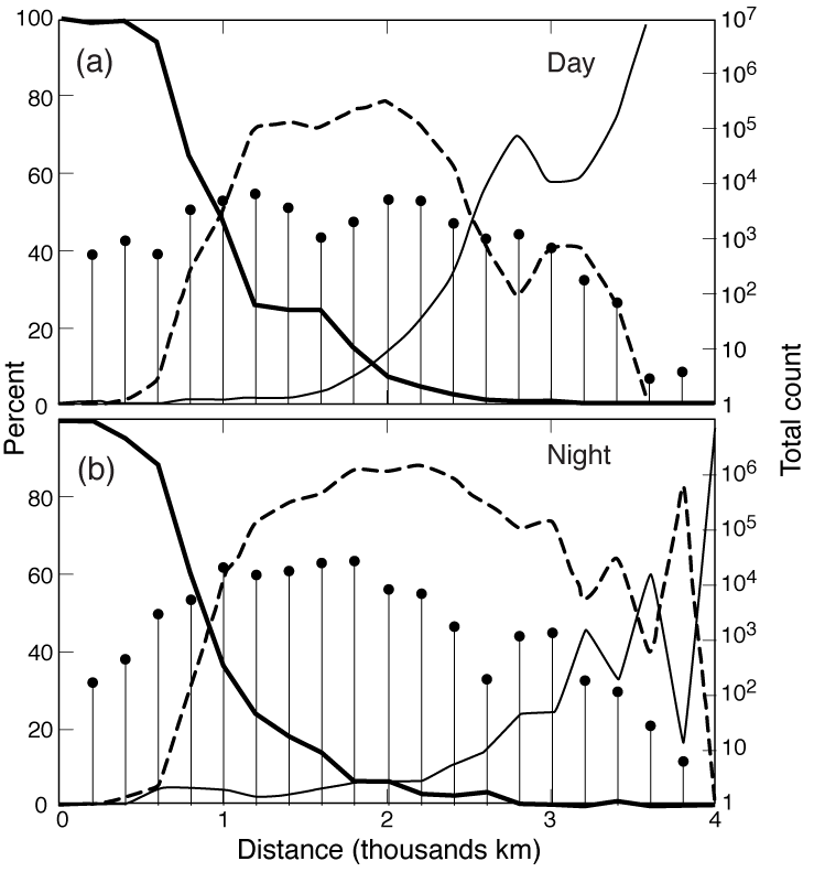
Figure 6. Percentage of different propagation types as a
function of distance for (a) day and (b) night. Thick solid line is
for ground wave, dashed for first-hop sky-wave, and thin solid for
second-hop sky-wave. The bars indicate the total number of strikes
detected in each 200 km distance bin (right ordinate).
Timing errors were calculated by time-correlating data from the PacNet test sensor with NLDN data and comparing speed-of-light propagation time (determined from the NLDN stroke time and the known propagation distance) with the arrival time measured by the sensor (Fig. 7). These histograms were obtained by measuring the arrival-time delay of PacNet sensor reports relative to NLDN estimated stroke times measured with an accuracy of approximately one microsecond. All reports from one week of observations are included in this analysis. Figs. 7a and c include reports with the same polarity as the NLDN peak current, and Figs. 7b and d include opposite-polarity reports. The polarity reversal (relative to the polarity determined by the NLDN) occurs when the earlier signal components (ground wave, then 1st-hop, then 2nd-hop) fall below the fixed detection threshold of the sensor. The ground wave signal delay distributions (average and standard deviation sigma) were nearly the same for day and night (Figs. 7a, c). The first-hop sky-wave distribution shift from daytime to night-time value can be seen in Figs. 7b and d. The second-hop distribution shift from a daytime value to night value is seen in Figs. 7a and c. Note that the polarity reversal of the first hop helps distinguish it from the ground-wave and second-hop signals, and that the signals delay distributions have almost no temporal overlap.


Figure 7.(a) Daytime ground wave signal delay distribution is
centered at 20.0 µs and has a standard deviation of 5.0
µs. Second-hop sky wave distribution is centered at 90.0
µs (sigma=5.1 µs). (b) First-hop (inverted) sky-wave
distribution is centered at 52.9 µs and has a standard
deviation of 4.7 µs (graph inverted in reference to reversed
polarity of first hop). (c) Night-time average for ground-wave
distribution is 19.3 µS (sigma=4.7 µS). Second-hop wave
centered at 104.0 µS, with sigma=8.0 µS. (d) First-hop
distribution is centered at 70.5 µS with sigma=4.0 µS
(graph inverted in reference to reversed polarity of first
hop).
Angle errors were calculated by time-correlating data from the test sensor with NLDN data (150 µs time window) and comparing the true azimuth from the sensor (determined from the NLDN stroke location) with the azimuth measured by the sensor. An angle error histogram was derived from all time-correlated events with signal strengths from just above threshold to four times threshold (Fig. 8). The parametric fit has a mean value of -4 degrees (resulting from an uncorrected antenna rotation and site errors due to local site conditions), and a standard deviation of 4.5 degrees. This value is conservative since it includes polarization errors and the variation of the local site error around its mean value.

Figure 8. Angle error without site-error correction has a mean
value of -4.0 degrees and a standard deviation of 4.5 degrees (for
both day and night).
Propagation characteristics between two widely separated locations (both signal attenuation and phase changes as a function of frequency) transition fairly continuously from the daytime to the nighttime behavior, over a period of 2-3 hours. This fact has been confirmed through analyses of arrival-time delay and relative amplitude as functions of time-of-day for a portion of the PacNet sensor test period. For one 48-hour observation period (hours 96 through 144), all lightning was at least 900 km from the test sensor (diamond symbols in Fig. 9). The plateau in the time-delay time series (Fig. 9a) at ~50-55 µs reflects the behavior during daytime propagation when the D-layer extends lower in the ionosphere (e.g., Fig. 1). The plateau at ~70-75 µs reflects the behavior during nighttime propagation. Note the rapid and smooth transition between the two stable conditions that occurs during day-night transitions.
The PacNet "current" estimate (Fig. 9b) employed the propagation model, using an attenuation rate of 10,000 km (representative for daytime propagation). This value is typically between 0.5 and 1.0, with random variations that can be larger than the day-night variability. The extent of these random variations is correlated with the variation in propagation distance, as one would expect. Note that for the hours 132-144, when most of the lightning is in the (narrow) range of 1500-2500 km, the random variability gets rather small. We note that this is the "sweet spot" range for one-hop propagation (see Figs. 5 and 6).

Figure 9. Time-series plots of (a) the variation of arrival-time
delay of VLF signals observed by the PacNet test sensor in Tucson,
AZ relative to GMT time-of-occurrence of the CG stroke determined
by the NLDN. Each symbol represents the median value of nine
time-ordered events. (b) Peak current estimated using the PacNet
sensor magnetic field peak, relative to NLDN estimated peak
current. Diamonds in the lower part of each figure show the
distance of the events from the sensor (right ordinate).
In addition, the behavior of PacNet DE during the transition periods between night and day over the Pacific was investigated, using the LLDN. Ground waves from flashes within 800 km of Hawaii were used as reference data. The two Hawaii sensors detected these events and the ground wave propagation was assumed to have no diurnal variation. The same events detected by distant sensors (excluding Hawaii sensors) were assumed to be sky waves, since all other sensors were more than 2400 km away. Hourly relative DE values were obtained by comparing the number of sky wave events to the number of ground-wave events near Hawaii (Fig. 10). In Fig. 10, the nighttime maximum DE begins to drop at ~0300 Hawaii local time, when the U.S. west coast sensors are in dawn. The lowest DE is reached at 0600 LT when the whole path from Hawaii to North America is in daylight. This continues until 1500 LT, when the North American sensors reach the dusk, and DE starts to enhance. The maximum DE is reached at 1800 LT when the whole propagation path is on the night side again. The relative DE during the day drops to ~20% of the night value. It should be noted that the diurnal variation shown in Fig. 10 over this test configuration area near Hawaii is close to its upper limit, as the nearest non-Hawaii sensors are >2400 km away. For quantitative applications of the PacNet data stream, such as numerical modeling, a linearly interpolated curve can be fit to the observed diurnal variation.
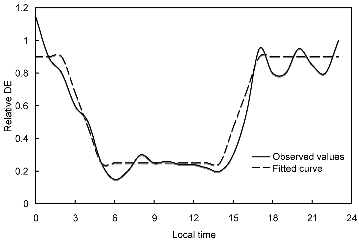
Figure 10. Empirically derived diurnal DE variation over the
North Pacific (solid line) and fitted curve used for diurnal DE
correction (dashed line). Since the actual DE of ground-wave events
is not exactly known, the DE-scale (y-axis) is relative.
Acknowledgments: We are grateful to James Weinman for his encouragement to undertake the development of PacNet, to Joseph Nowak for help with detector site selection and installation, and to Nancy Hulbirt for assistance with graphics. This work is supported by the Office of Naval Research under grant numbers N00014-08-1-0450 and N00014-05-1-0551.