(originally designed for SIO Visualization Introductory Class)
Quick Contents:
I. Obtaining
and
Visualizing Topography Datasets
Tools: GMT & Dmagic (Fledermaus)
II. Assembling Quicktime Movies
Tools: ImageReady
III. Displaying multiple movies & files
Tools: iMovie
IV. Recording sound/narration
Tools: GarageBand, iTunes, & iMovie
Tools: GMT & Dmagic (Fledermaus)
II. Assembling Quicktime Movies
Tools: ImageReady
III. Displaying multiple movies & files
Tools: iMovie
IV. Recording sound/narration
Tools: GarageBand, iTunes, & iMovie
Helpful
Links: Kurt
Schwehr's 2003 Class Notes
and Blog
Kerry Key's 2004 Class Notes (pdf)
SIO Viz Center Tutorial
SRTM30Plus Fledermaus sd files
Fledermaus installation contact: vizinfo@ucsd.edu
Kerry Key's 2004 Class Notes (pdf)
SIO Viz Center Tutorial
SRTM30Plus Fledermaus sd files
Fledermaus installation contact: vizinfo@ucsd.edu
I. Obtaining and Visualizing Topography
Where can I obtain topography data?
This new global dataset, provide by SIO's very own JJ Becker and David Sandwell, is a good place to start. Detailed information about the dataset is provided at the above link. In short, this dataset combines the land topography from NASA's SRTM with Smith and Sandwell ocean topography data and uses GTOPO30 data for high latitudes. Resolution of this data is roughly 1 kilometer (or 30 arc seconds).
To acces this data, click on the above link, then click on the link "FTP SRTM30_PLUS". This will mount an ftp site on your desktop where you can access the data.
- README.txt file: contains a ton of useful information about the data and how to prepare it for a useful application.
- DATA directory: contains gzipped files of binary topography data. Naming convention (see README.txt in this folder) is as follows: e020n40 is a region with the northwest corner at 20E 40N, and is implicitly 40 degress wide and 50 degrees tall. The antarctic data sets are 60 wide and 30 tall.
- GRD directory: contains bin2grd script for converting binary data into grd-netcdf format. Also contains make-all.com, an example script showing usage of bin2grd command (very useful!).
Note that other topography data sets exist, some with much higher resolution, although without complete global coverage:
NASA's SRTM dataset README .txt file for xyz2grd conversion
How do I get
topography data into a usable format?
To begin, drag bin2grd and make-all.com (grd directory) to a working space on your computer. Next, drag the topography data file (data directory) of your region of interest to your computer. If you need more than one of these files, drag all necessary.
As an example, lets use California as our study region and grab file w140n40.Bathmetry.srtm.gz from the ftp site.
First we want to decompress the data:
% gunzip w140n40.Bathmetry.srtm.gz
Next we need to convert the data from 16 bit binary to a grd-netcdf file. To do this, we can cheat by inspecting the commands in the make-all.com file and running the one appropriate for our data file:
% bin2grd w140n40.Bathmetry.srtm -140 -100 -10 40
Note that bin2grd contains the GMT command xyz2grd, a command commanly used to convert an xyz data file to a grd file. For more information on xyz2grd, type 'man xyz2grd' and 'more bin2grd'.
You should now have a file called w140n40.Bathmetry.srtm.grd. Now we can manipulate the grd file in a variety of ways. First we'll chop off some of the data since we're just interested in California topography. To figure out what the current dimensions of the file are, type:
% grdinfo w140n40.Bathmetry.srtm.grd
This should give some vital statistics about the file, including the min/max of the x,y, and z values, in addition to the x,y increments and the number of x,y grid cells:
w140n40.Bathmetry.srtm.grd: x_min: -140 x_max: -100 x_inc: 0.00833333 units: user_x_unit nx: 4800
w140n40.Bathmetry.srtm.grd: y_min: -10 y_max: 40 y_inc: 0.00833333 units: user_y_unit ny: 6000
w140n40.Bathmetry.srtm.grd: z_min: -6031 z_max: 4228 units: user_z_unit
w140n40.Bathmetry.srtm.grd: scale_factor: 1 add_offset: 0
California is roughly defined by lat = 32.5 - 40 and long = -125 - -114. We will use the GMT command 'grdcut' to chop this grid down to size to make a new grid called California.grd. (for more info on grdcut, type 'man grdcut'):
% grdcut w140n40.Bathmetry.srtm.grd -GCalifornia.grd -R-125/-114/32.5/40
Note: if you have more than one topography data file that you need to merge together, you can use the 'grdpaste' command to easily do this as long as the two files have one comman edge (for more info on grdpaste, type 'man grdpaste').
How
do I use topography to create 3D scenes?
Now we are ready to import this California.grd into Dmagic, part of the Fledermaus package. Dmagic can be found under Applications/IVS Fledermaus/. Open up the application and start a new project:
--> Project --> New Project (give location of working space on your computer)
Next we will import the topography data:
--> File --> Import Surface (select the location where you have stored California.grd)
--> File type: GMT GRD / NETCDF
--> Scan for information (check information for consistency with grdinfo command)
--> Surface interpretation: Output a DTM (.dtm)
--> Convert & Save (name the .dtm file)
You now should have two files appear under Data Components: name.dtm & name.geo. To view these files, highlight the .dtm file and click on the '>' button on the right side of the Data Component panel.
More than likely, the colorbar values will not correspond to the z-values of your grd file. To fix this, click on Color Map Editor:
--> Hight Dependent CMap
--> Max (enter max z-value)
--> Min (enter min z-value)
--> Resample
--> Okay
To refresh, click on '>>' .
To use an alternative colormap, click on CMap Librarian (located under the colorbar). For this example, we'll choose gmtglobe_d.cmap.
Next, we shade. Click on Surface Shader. Play with the direction and magnitude of shading in the Shadow Direction panel. Click on Start Rendering to preview shade and Save Shade to finish. Close.
Almost done. The last step is to click on Assemble Fledermaus Objects. Defaults should be fine. Note that the final object file will be called name.sd. Click on Build Object. Close.
Now we will run Fledermaus. Click on Run Fledermaus for a shortcut to the application. Use the widgets and scroll bars to manipulate the view of your newly created scene.
To save your scene:
--> File -->
Save Scene
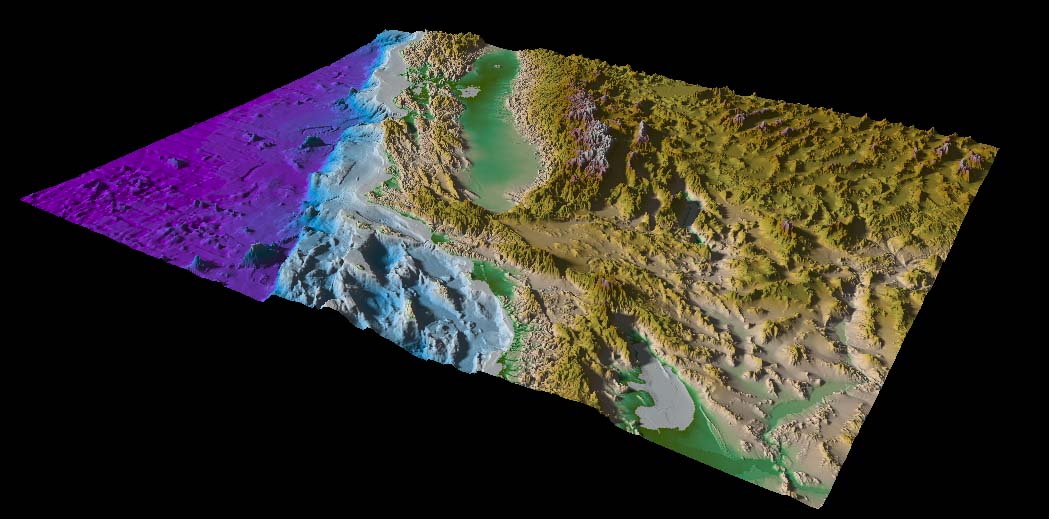
An example:
An example:
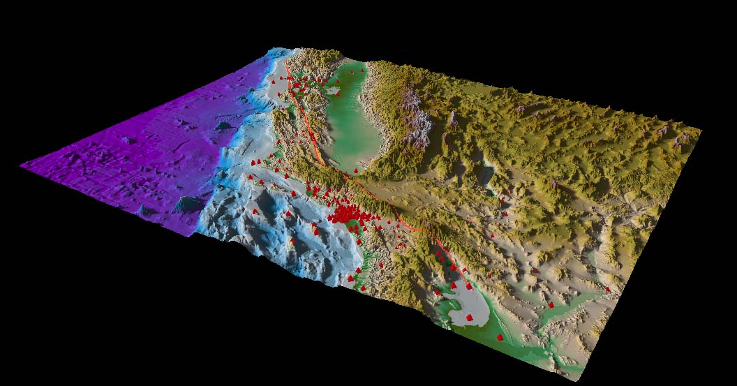
How do I add points and lines to the scene?
Adding lines or points to your Fledermaus scene can be done from the command line. You need a file containing x,y pairs of points. Click here to obtain an example of a list of points representing the San Andreas Fault (saf.xy). Make sure that your own file contains a 9999 9999 marker on the last line. The following command can be used to transform these points into a line file readable by Fledermaus (an .sd file):
% cmdop mklines -in saf.xy -out saf.sd
Now we will add this fault file to the topography scene in Fledermaus:
--> File --> Open Data Object --> saf.sd
Make sure that cafaults.sd is highlighted in the lower left box and click on Drape Lines under Line Height Controls. You can also adjust the line size and color in the Line Display Options box.
Next we'll convert a file containing GPS station locations (gps.xy) into an .sd file and add these to the topography scene:
% cmdop mkpoint3d -in gps.xy -out gps.sd
Now we will add this gps station location file to the topography scene in Fledermaus:
--> File --> Open Data Object --> gps.sd
Click on Drape Points to drap these x,y points over the topography. Adjust the size of the points with Point Radius, the shape with Marker Type, and the color with By Color.
To save your scene:
--> File --> Save Scene
Another example:
How
can I drape a scalar grid over topography?
Suppose that you have a topography grd (topo.grd) file containing elevation information for the 'z' component. In addition, suppose that you have a companion grd file containing some scalar "data" for the 'z' component that you want to display (ie., displacement). To colorcode the topography according to this new dataset (displacement.grd), repeat the steps described above for importing topography and the following additional steps for importing the scalar data:
--> File --> Import Surface (select the location where you have stored displacement.grd)
--> File type: GMT GRD / NETCDF
--> Scan for information (check information for consistency with grdinfo command)
--> Surface interpretation: Output a Scaler (.scaler)
--> Convert & Save (name the .scaler file)
To shade, click on Surface Shader. Under Selected Components, click on Overlay Scaler. Play with the direction and magnitude of shading in the Shadow Direction panel. Click on Start Rendering to preview shade and Save Shade to finish. Close..
Repeat Assemble Fledermaus step and launch Fledermaus. Often times exaggeration for the new .sd scaler draped file will need to be adjusted. In the Exag. box, change to 0.01 and hit return.
An example of horizontal displacement due to the 1906 San Francisco earthquake, drapped over topography:

How do I create a movie scene file?
To create a movie, you need to use
both Fledermaus and the Fledermaus MovieClient application, which is
part of the Fledermaus suite, but a separate executable.
For more info, also check out the Viz Center online
tutorial.
First you'll need to save your Fledermaus creation (collection of .sd files) into a .scene file.
--> File --> Save Scene
Next you'll need to create a flight path in Fledermaus using your scene and the widget control:
--> Controls --> Movie Controls.... --> Record
After clicking on the Record button, use the widget and scroll bars to visualize your scene. Click Stop when complete. Then save the flightpath:
--> File --> Save Flightpath
Next launch Fledermaus MovieClient (/Applications/IVS Fledermaus/Movieclient) and choose the scene and the flight path that you want to display. Click OK (you don't have to smooth, it gives you funny results, even makes the flight jerkier), then select the Movie Format, and change Frame Size if necessary, otherwise the default values work just fine. You can choose either mpeg or image sequence for your movie. Choosing image frames will generate a series of frames that you can assemble in Adobe's ImageReady and edit as needed.
II. Assembling Quicktime Movies
Stand-alone Quicktime movies can easily be made from a series of image files (ie. jpg, tiff, ps) and the Adobe Photoshop application ImageReady.
All image files must be placed into
a common folder before assembly process can begin.
Next, launch Adobe application ImageReady, which can typically be found under /Applications/Adobe Photoshop/ .
--> File --> Import --> Folder as Frames
Frames appear in Animation Window and can be rearranged as needed (drag n drop). Each frame can also be edited (add text, adjust color, etc.) just as a regular image file would be edited in Photoshop.
To adjust the timing of each frame, modify the menu under each frame labeled 0 sec. One second per frame is a good rate to begin with -- modify as needed for your own application.
To preview your movie, click on the '>' button at the bottom of the Animation Window.
To save your movie:
--> File --> Export Original --> Quicktime Format
The default Compression is usually optimized, although sometimes it helps to adjust the Quality of frames to Best.
For playback, simply open your new movie in Quicktime and play.
Click here for a really boring example of a short (short) movie, edited in ImageReady and saved as Quicktime movie.
Click here for a much more exciting movie, also edited in ImageReady.
III. Displaying Multiple Movies and Files
If you have multiple files, animations, and movies that you want to demonstrate, it may be useful to combine all of these into one single movie using Apple's iMovie software. An advantage of doing this is not only convenience (you don't have to worry about having multiple files open and running on multiple applications), but iMovie also allows you to add a creative edge to your final product (ie., sound, special effects). The only downside to creating one ensemble movie is file size -- you may want to keep an eye on this.
** NOTE: iMovie has a tendency to crash unexpectedly. Yuck. Save FREQUENTLY!!!!!!.
To begin, launch iMovie from the Applications folder. Next, open a new project:
--> File --> New Project
The next step is to begin importing files that you would like to display:
--> File --> Import
From here on out, I'd recommend just playing with the various tools and workspace at the bottom of the iMove project window. When you want to manipulate a file that has been imported, simply drag it to project workspace. You can apply special effects and transitions to each clip or photo and you can also adjust the speed of each of these through the turtle (slow) and bunny (fast) icons at the bottom . Sound effects can be added too (see next). Audio and sound clips can be imported in the same way and automatically appear at the bottom of the project workspace, typically highlighted in lavender. Often times the sound needs to be adjusted for each audio clip.
To save your movie project:
--> File --> Share
--> Quicktime Icon --> Compress movie for: Full Quality DV (no quality loss)
--> Share
IV. Recording Sound/Narration
To record special audio, the GarageBand application is fairly easy to use. Launch GarageBand from /Applications/GarageBand.
--> Create New Song --> Give name and location to save --> Create
Next create a new track:
--> Track --> New Basic Track
Now you're ready to begin. Click on the red circular button (record) and begin speaking into the microphone on your computer. When you are finished, click on the highlighted 'play' button to pause recording.
Now save your file:
--> File --> Export to iTunes
iTunes should now launch, and your recorded file should show up in a Source Directory, song titled My Song (or whatever you chose to name it). Your song will now be saved in a format (.aif) that iMovie can read.
Now return to iMovie to import the file:
--> File --> Import --> Locate your song in the iTunes folder
Your audio track should now appear at the bottom of your iMovie project workspace as a lavendar box. Clicking on the iMovie play button will allow you to play the sound on top of whatever visual files you have imported.
That's it -- good luck!